Spice up your plot
![]()
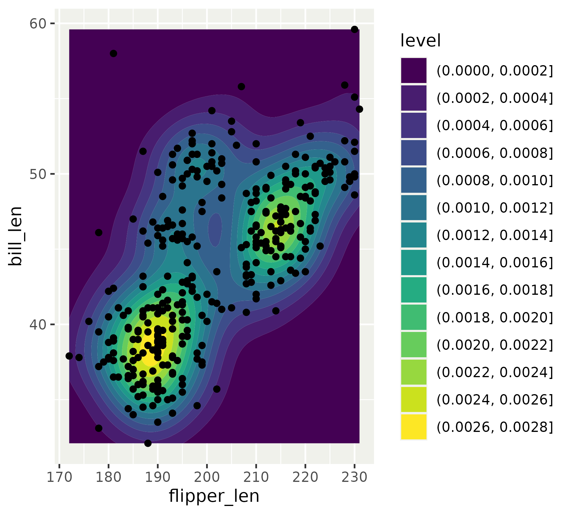
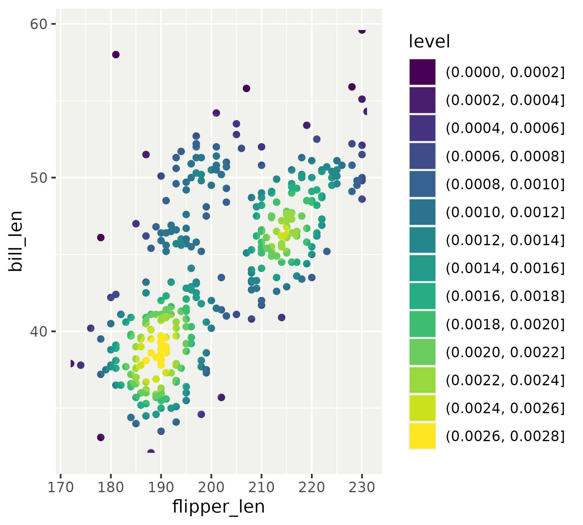
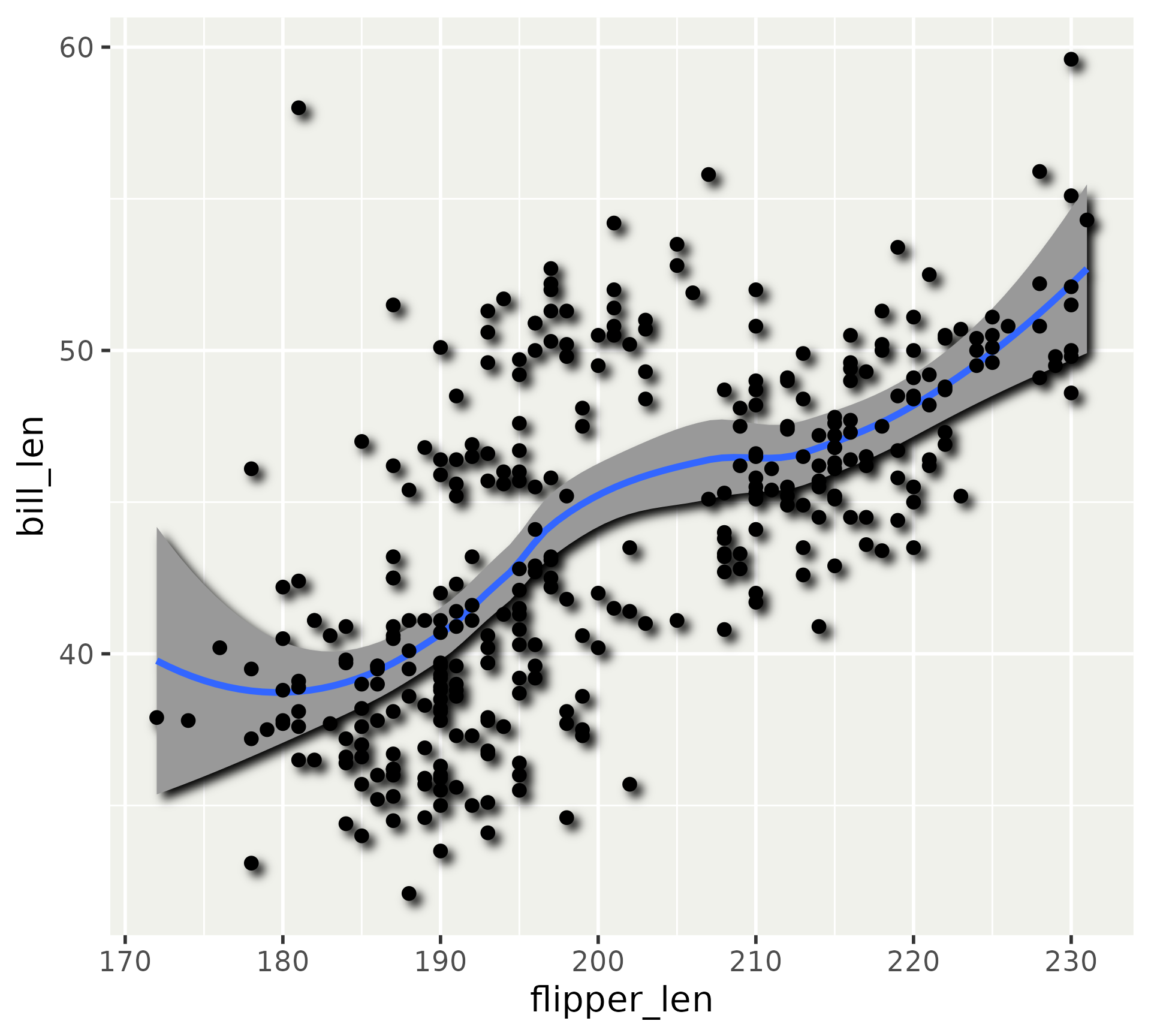
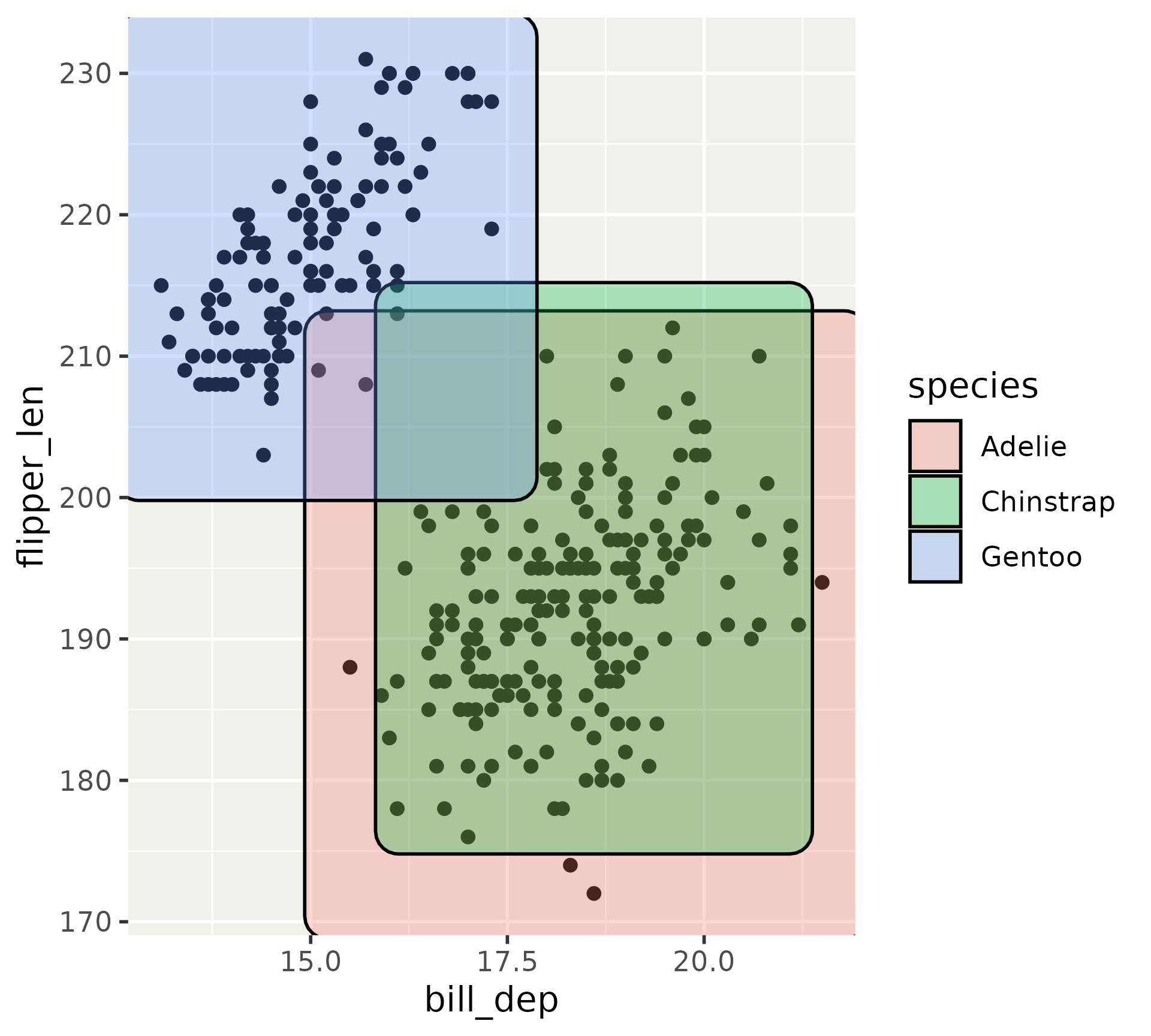
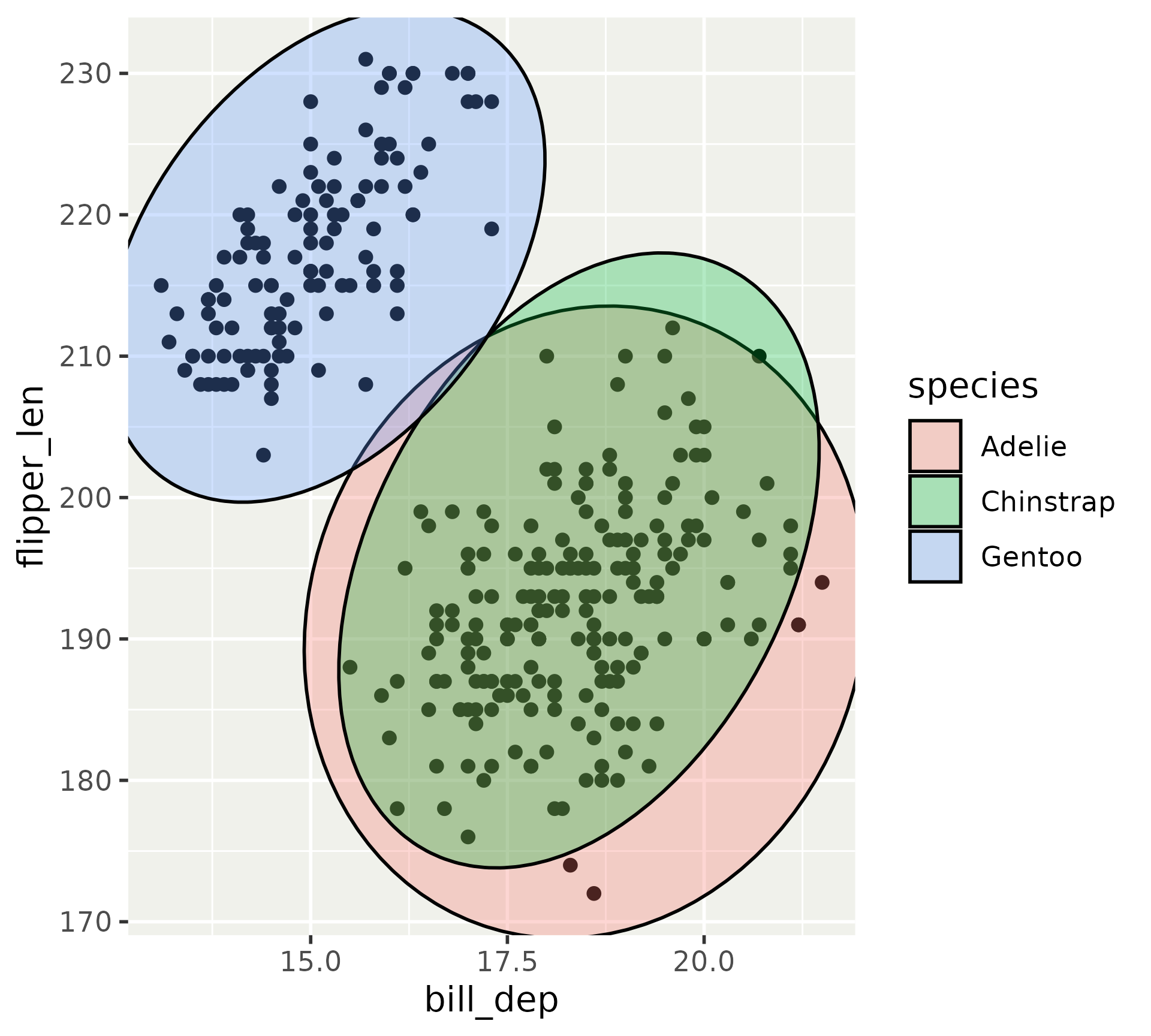
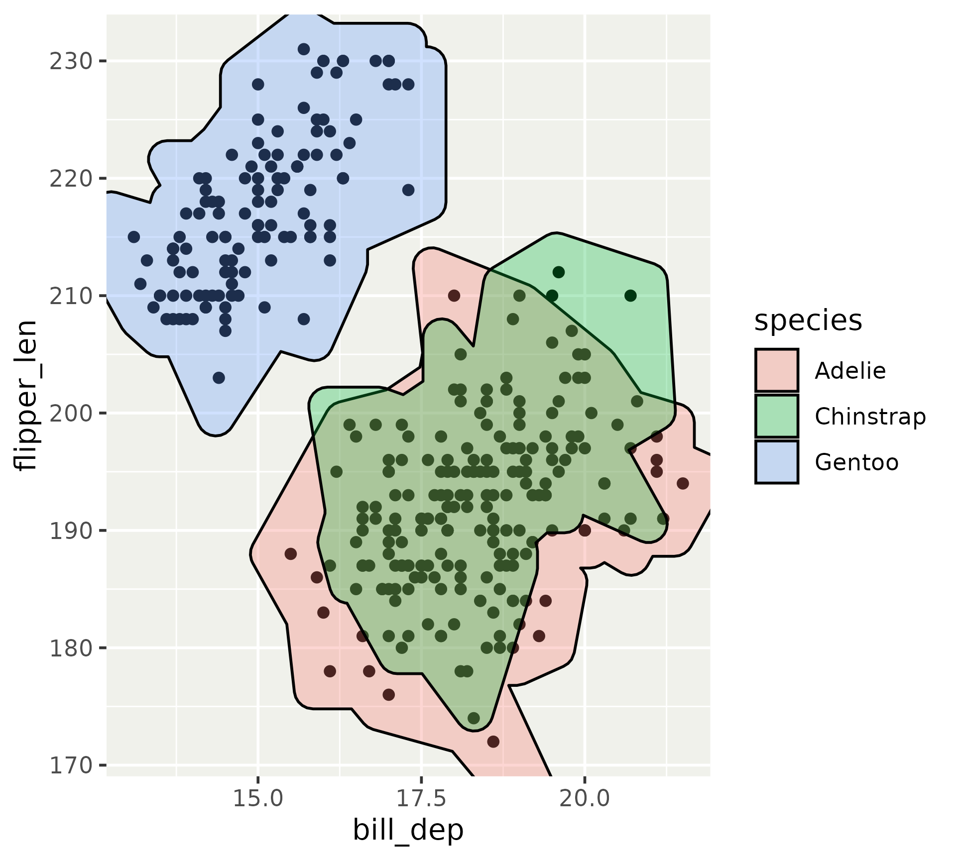
Filters
Filters
Filters
References
References
References

References
![]()
ggforce
- This is my grab-bag package. Expect some chaos
- Main focus on powerful building blocks
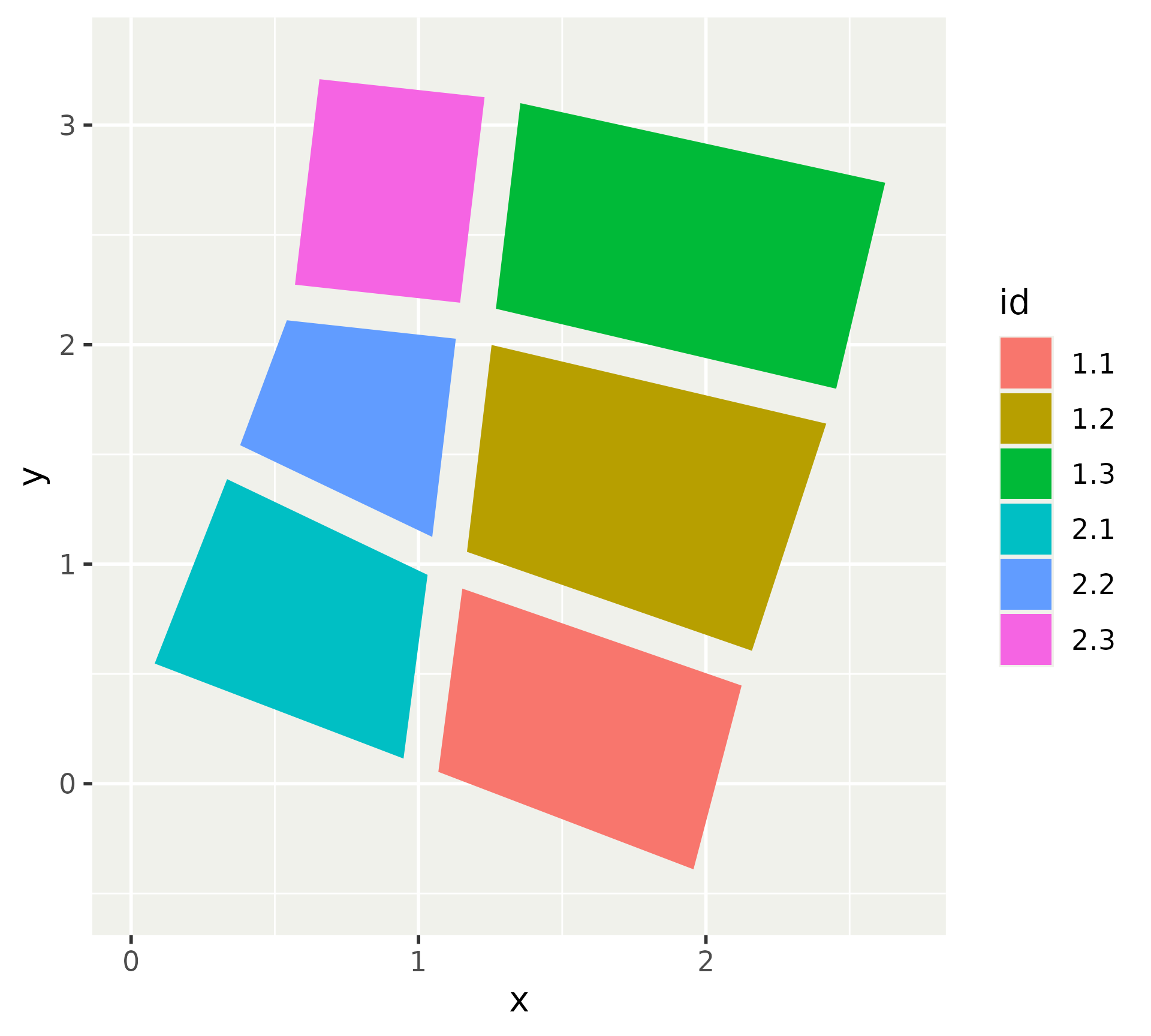
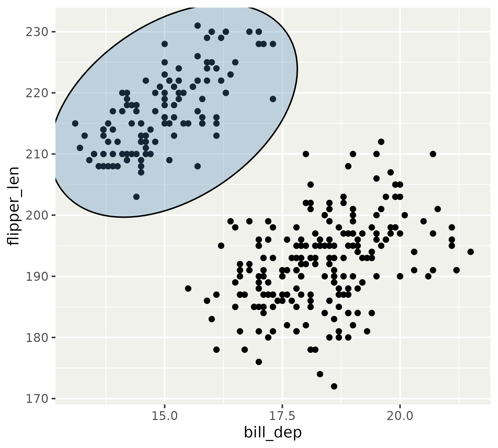
Shapes

Shapes
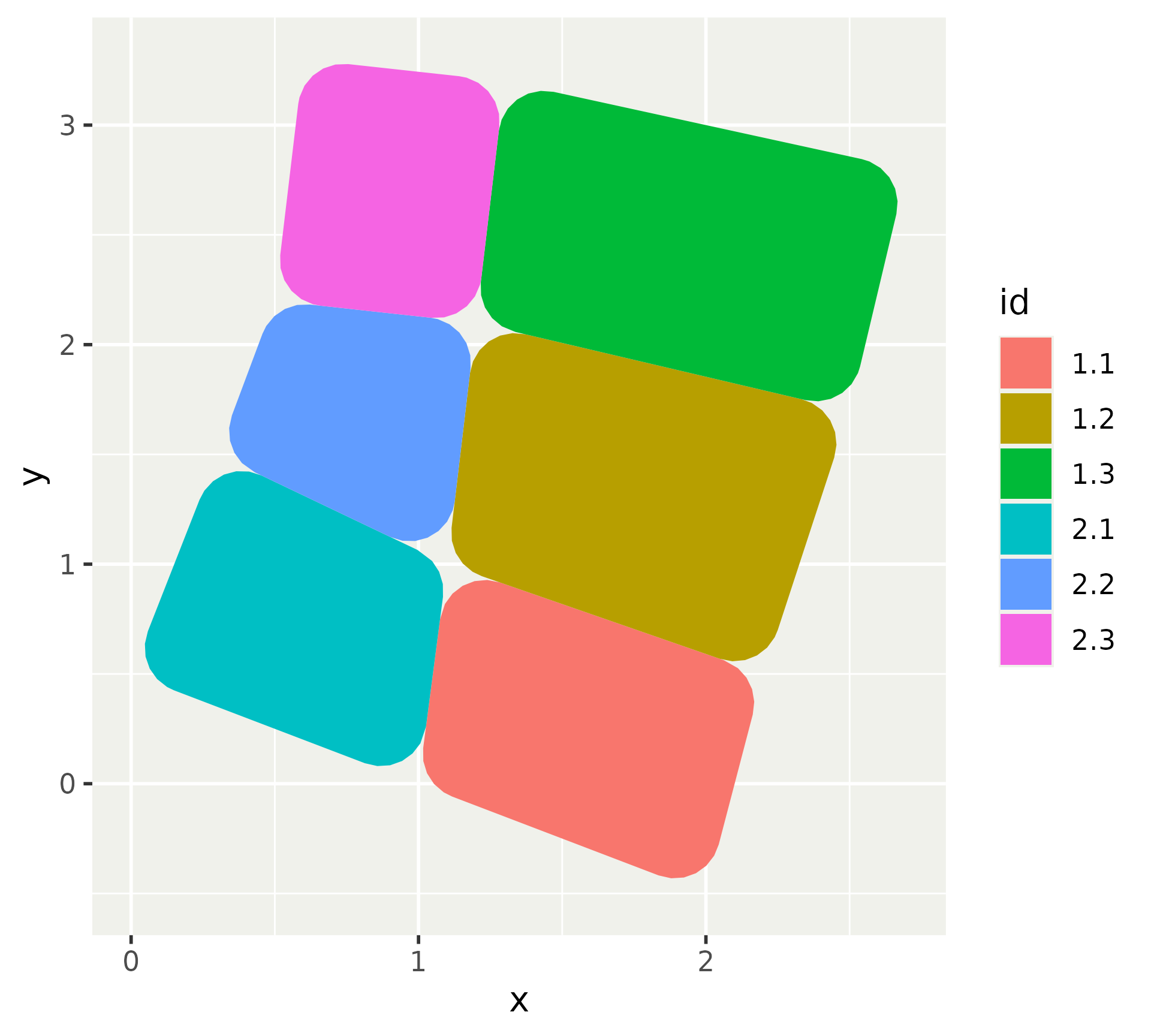
Shapes
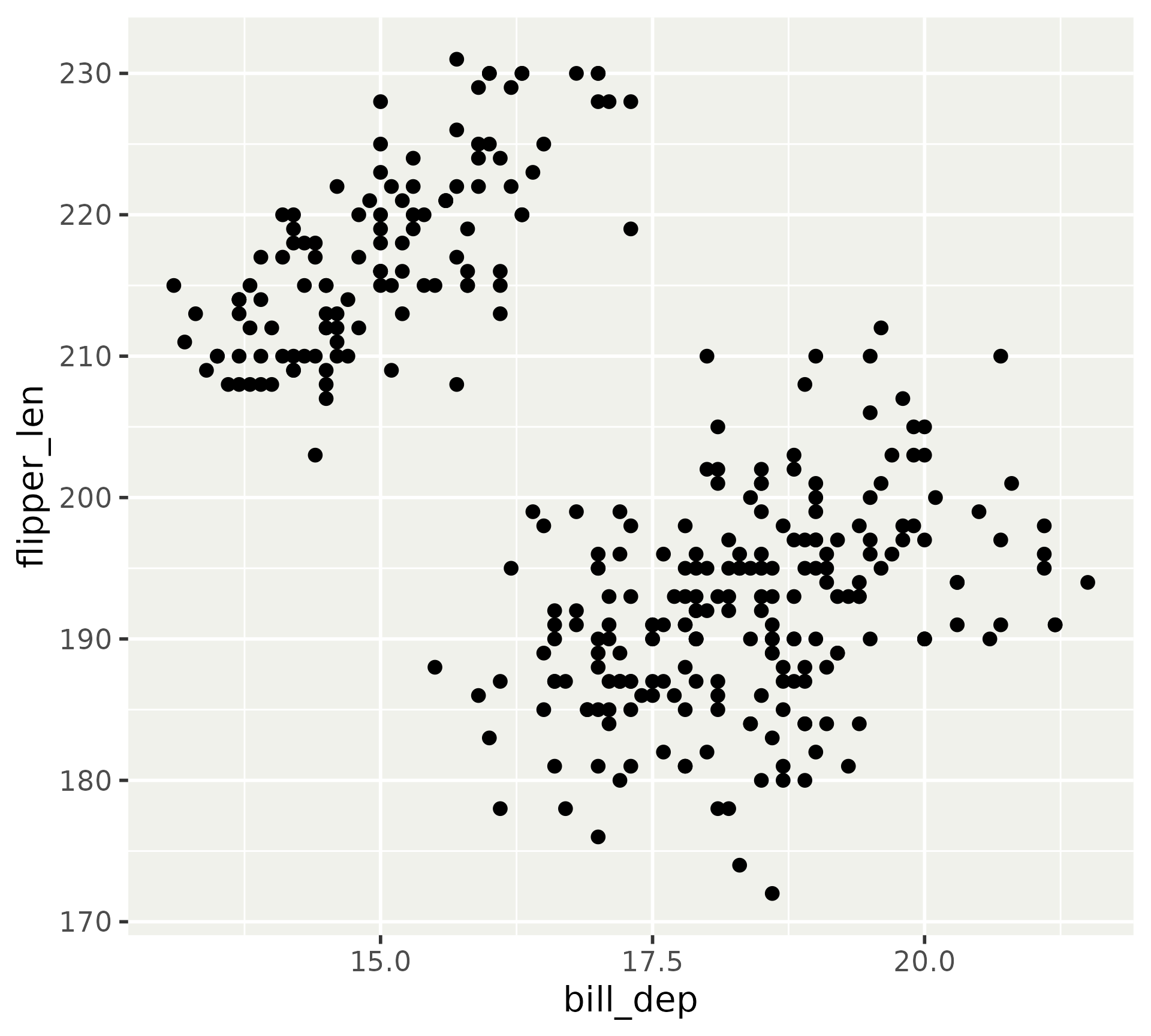
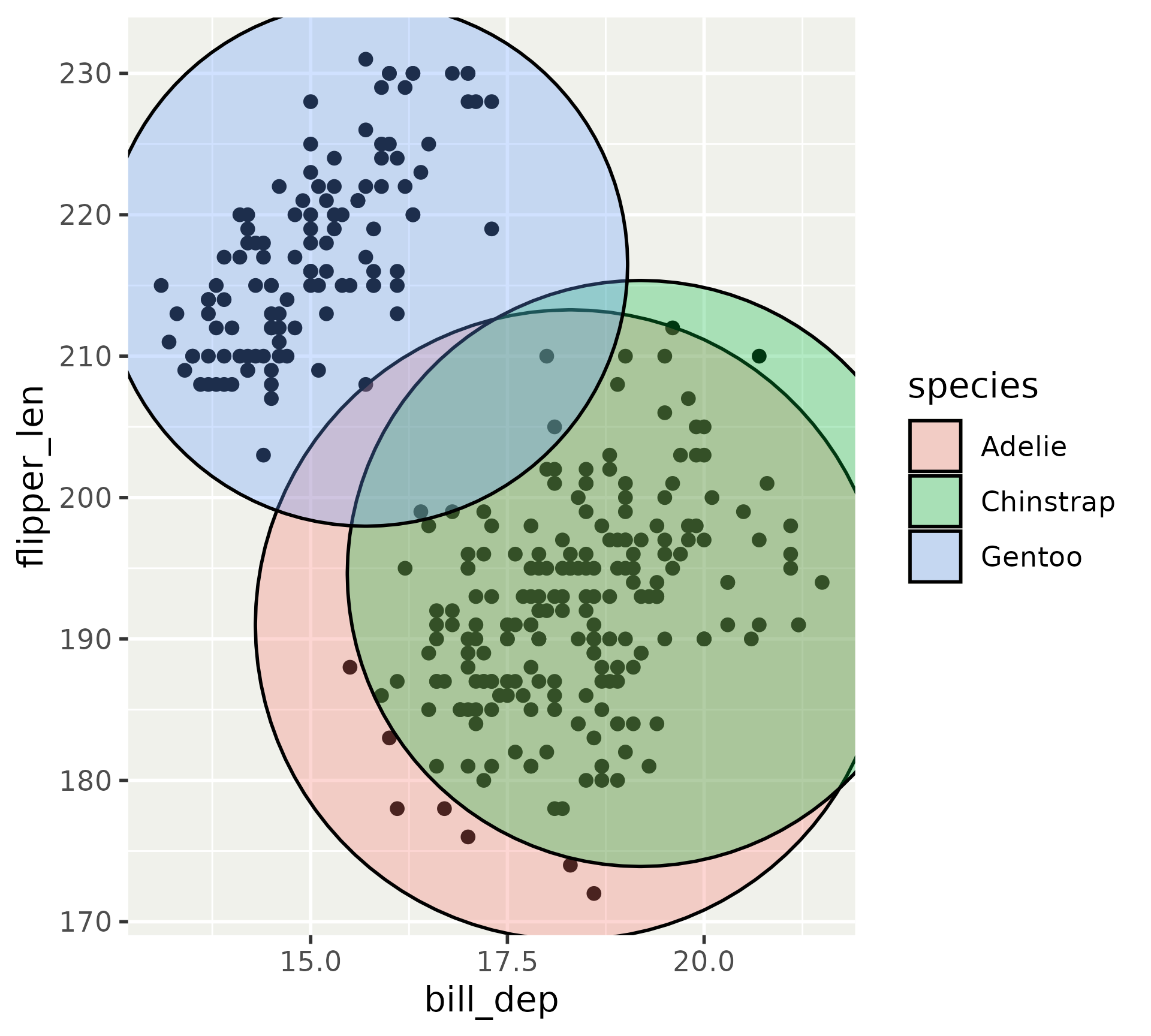
Marks
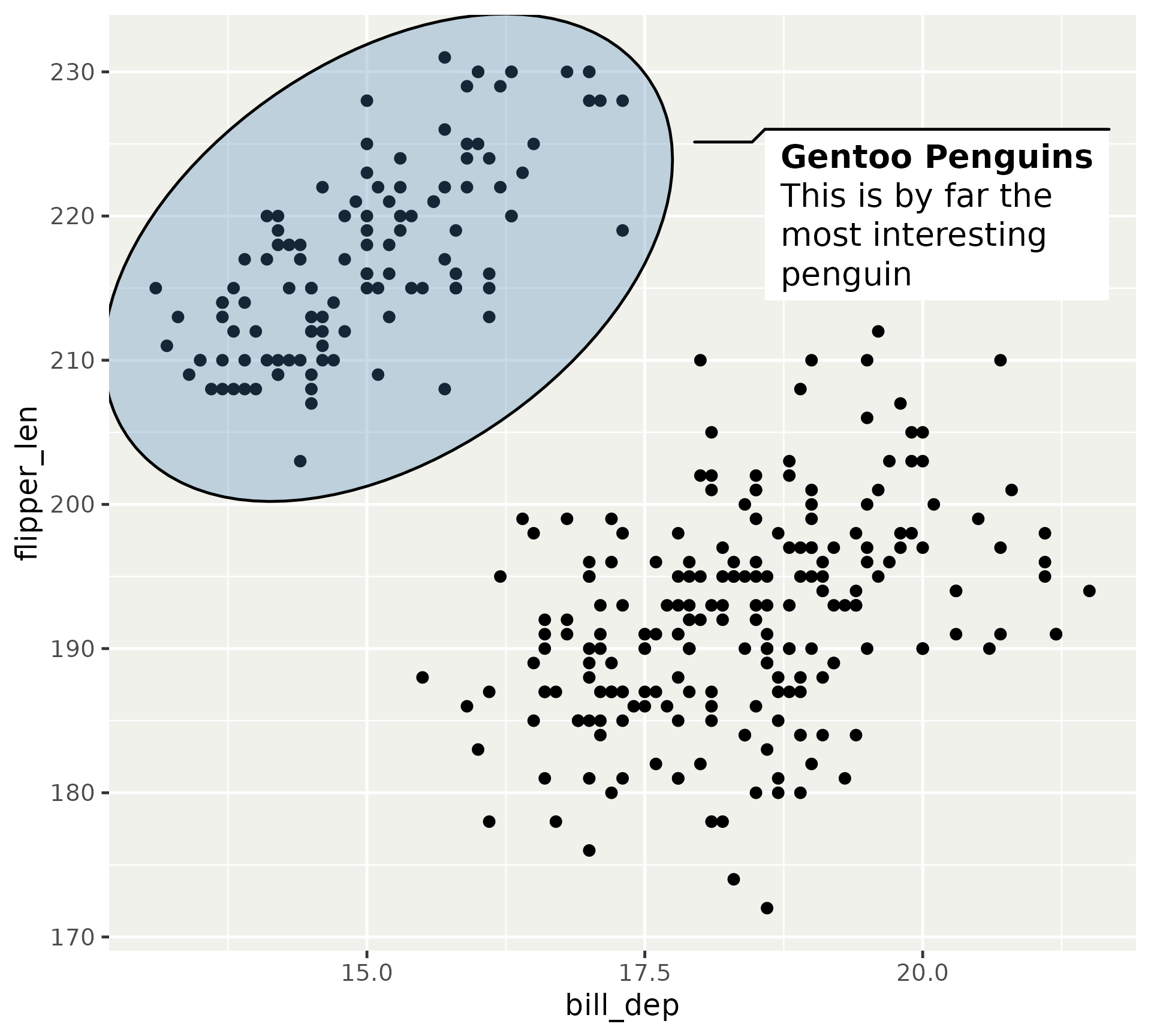
- The reason
geom_shape()exist - High-level annotation in plots
Marks
Marks
Marks
Marks
Marks
Marks
(geom_mark_*() is not yet marquee-aware)
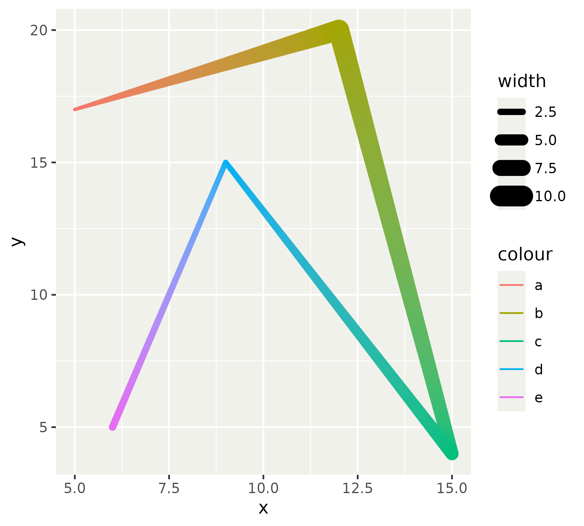
Links
- Supercharged
geom_segment()/geom_path() - Allows interpolation of aesthetics between anchors
# Lets make some data
lines <- data.frame(
  x = c(5, 12, 15, 9, 6),
  y = c(17, 20, 4, 15, 5),
  xend = c(19, 17, 2, 9, 5),
  yend = c(10, 18, 7, 12, 1),
  width = c(1, 10, 6, 2, 3),
  colour = letters[1:5]
)

ggplot(
  lines,
  aes(x = x, y = y, xend = xend, yend = yend)
) +
  geom_link(
    aes(
      colour = colour,
      alpha = after_stat(index),
      linewidth = after_stat(index)
    )
  )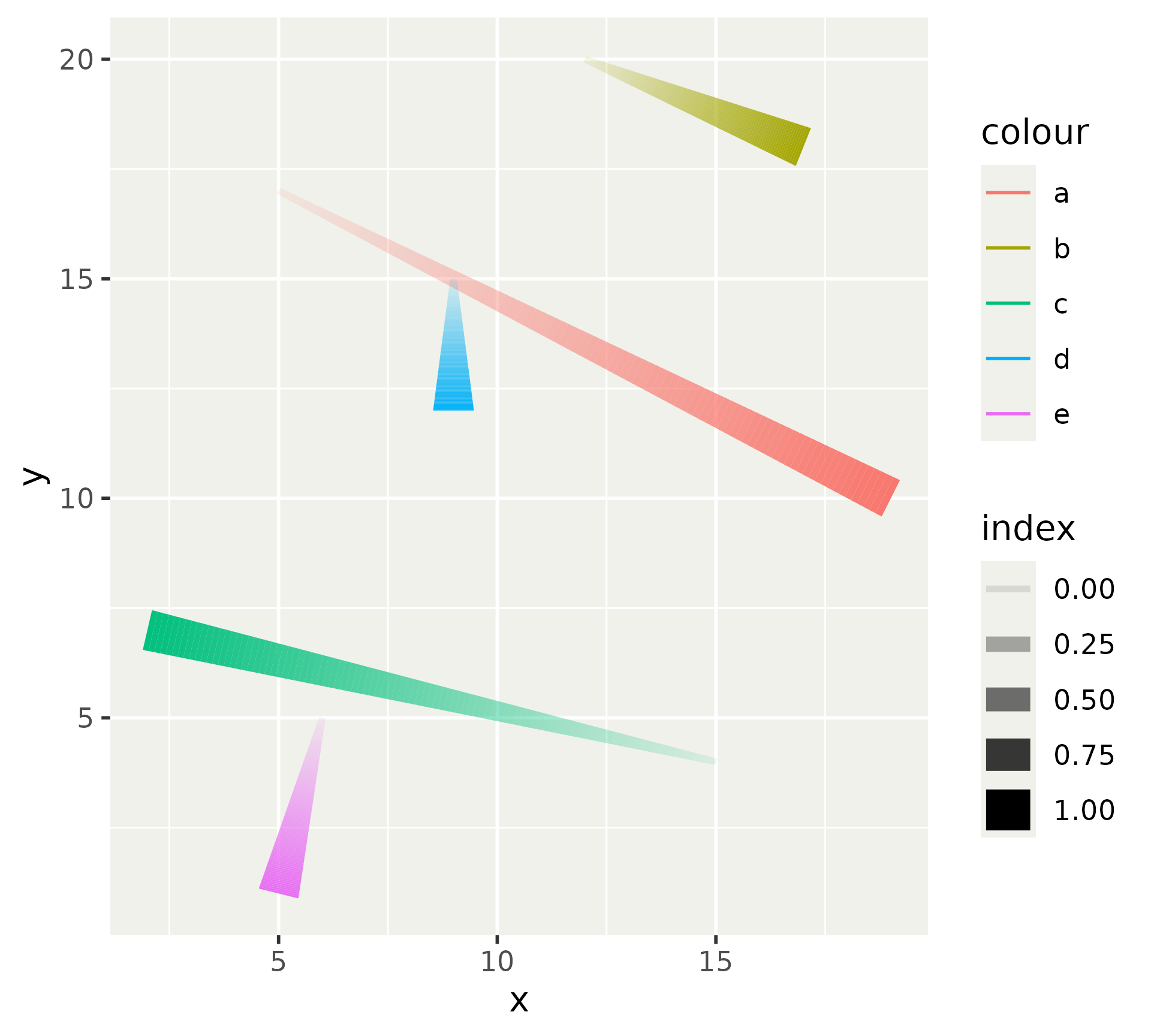
Links