Tree-based and ensemble models
Tree-based methods
Decision trees on their own, are very explainable and intuitive, but not very powerful at predicting.
However, there are extensions of decision trees, such as random forest and boosted trees, which are very powerful at predicting. We will demonstrate two of these in this session.
Decision trees
- Excellent decision Trees explainer web app by Jared Wilber & Lucía Santamaría
![]()
Classification Decision trees
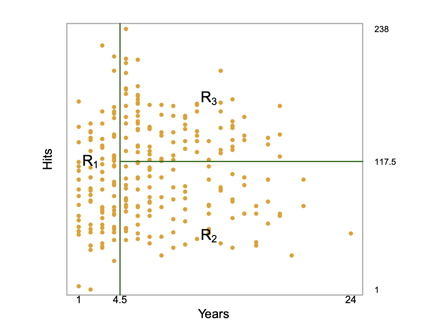
- Use recursive binary splitting to grow a classification tree (splitting of the predictor space into \(J\) distinct, non-overlapping regions).
![]()
Classification Decision trees
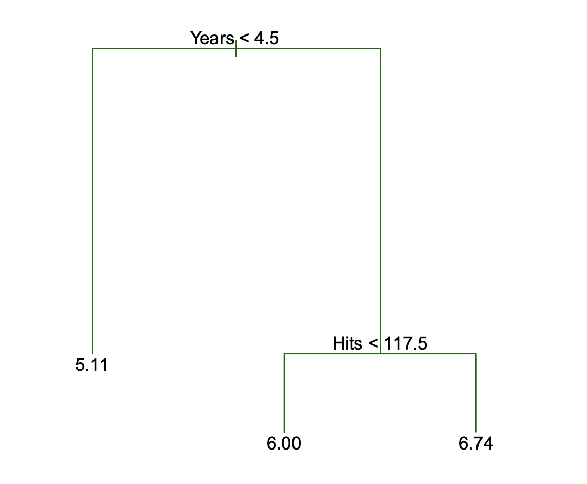
- For every observation that falls into the region \(R_j\) , we make the same prediction, which is the majority vote for the training observations in \(R_j\).
![]()
Classification Decision trees
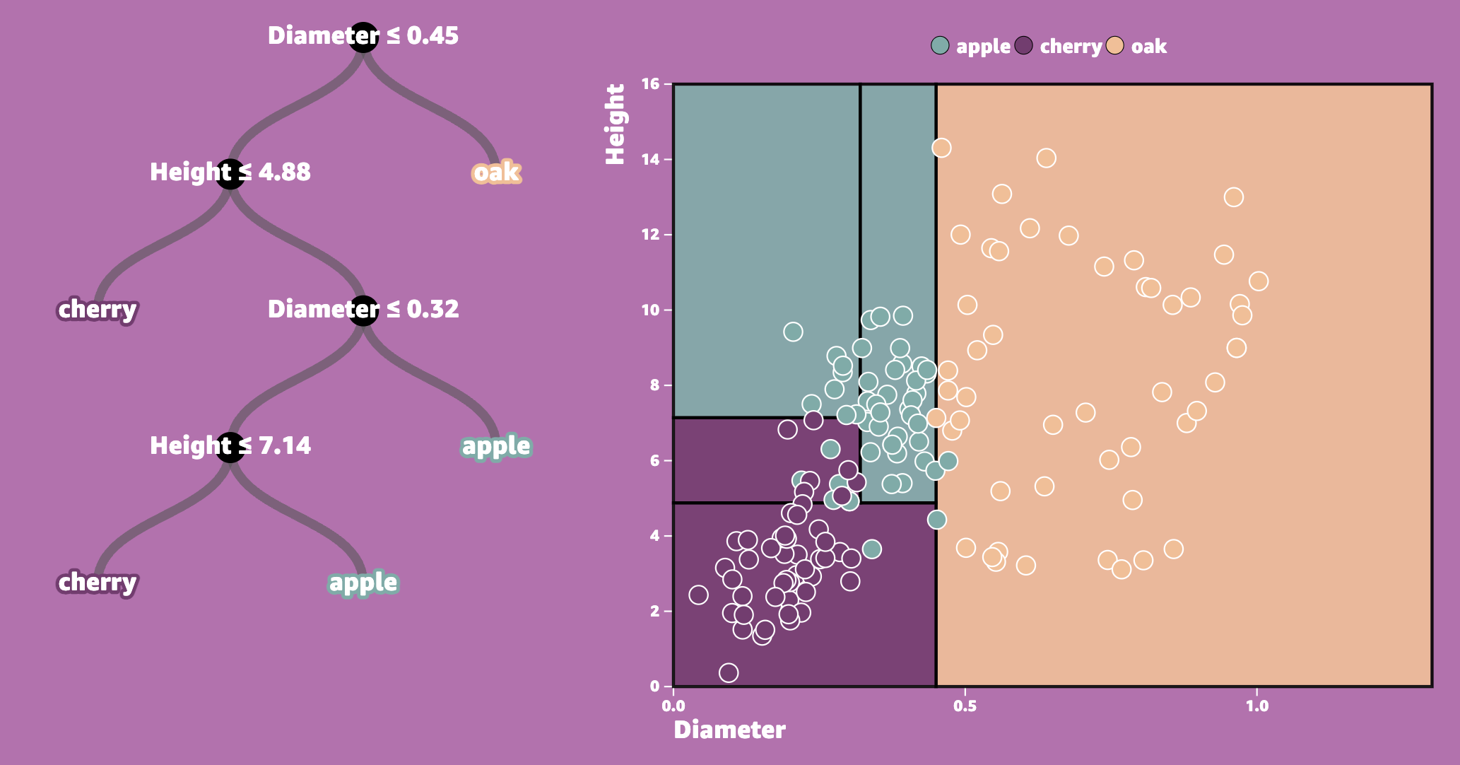
- Where to split the predictor space is done in a top-down and greedy manner, and in practice for classification, the best split at any point in the algorithm is one that minimizes the Gini index (a measure of node purity).
![]()
Classification Decision trees
- A limitation of decision trees is that they tend to overfit, so in practice we use cross-validation to tune a hyperparameter, \(\alpha\), to find the optimal, pruned tree.
![]()
Example: the heart data set
Let’s consider a situation where we’d like to be able to predict the presence of heart disease (AHD) in patients, based off 13 measured characteristics.
The heart data set contains a binary outcome for heart disease for patients who presented with chest pain.
Example: the heart data set (cont’d)
An angiographic test was performed and a label for AHD of Yes was labelled to indicate the presence of heart disease, otherwise the label was No.
Do we have a class imbalance?
It’s always important to check this, as it may impact your splitting and/or modeling decisions.
Data splitting
Let’s split the data into training and test sets:
Categorical variables
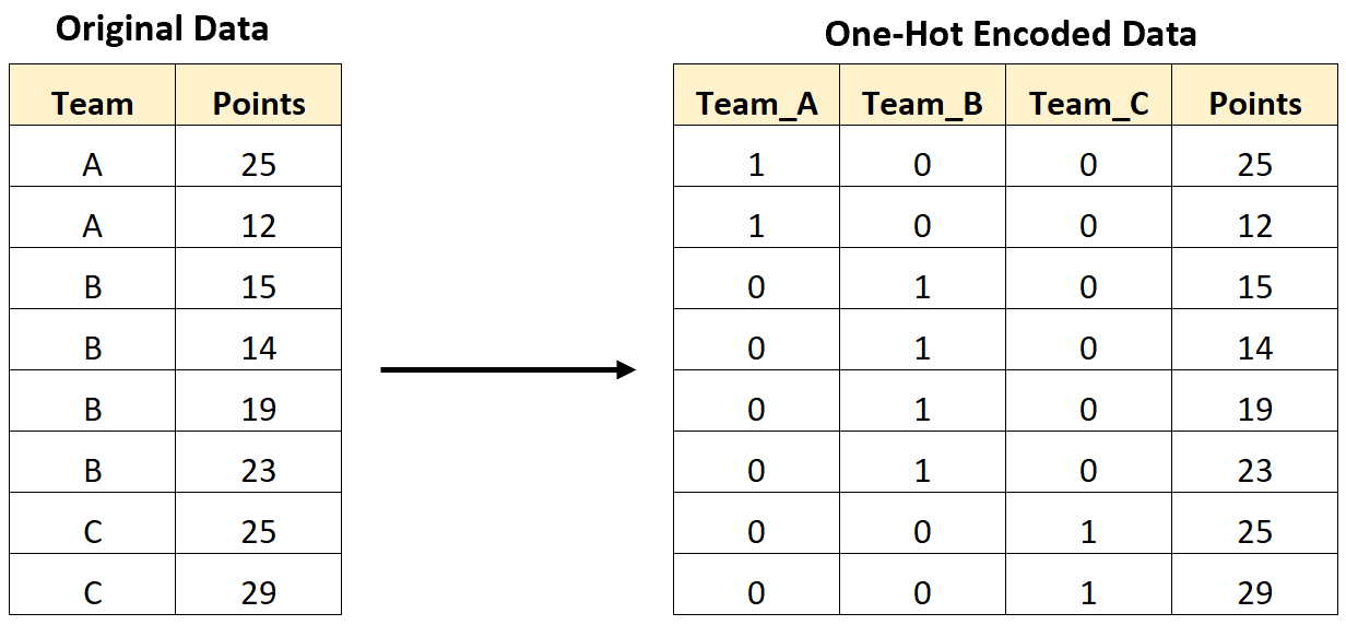
This is our first case of seeing categorical predictor variables, can we treat them the same as numerical ones? No!
In scikit-learn we must perform one-hot encoding
Look at the data again
Which columns do we need to standardize?
Which do we need to one-hot encode?
One hot encoding & pre-processing
handle_unknown = "ignore" handles the case where categories exist in the test data, which were missing in the training set. Specifically, it sets the value for those to 0 for all cases of the category.
Fitting a dummy classifier
Put the mean cross-validated error in a data frame
Add the mean cross-validated error to our results data frame
Can we do better?
We could tune some decision tree parameters (e.g., alpha, maximum tree depth, etc)…
We could also try a different tree-based method!
Another great explainer: the Random Forest Algorithm by Jenny Yeon & Jared Wilber
Random forest in scikit-learn
Add the mean cross-validated error to our results data frame
Can we do better?
Random forest can be tuned a several important parameters, including:
n_estimators: number of decision trees (higher = more complexity)
max_depth: max depth of each decision tree (higher = more complexity)
max_features: the number of features you get to look at each split (higher = more complexity)
We can use GridSearchCV to search for the optimal parameters for these, as we did for \(K\) in \(K\)-nearest neighbors.
Tuning random forest in scikit-learn
Comparing to our other models
How did the tuned Random Forest compare against the other models we tried?
Boosting
No randomization.
The key idea is combining many simple models called weak learners, to create a strong learner.
They combine multiple shallow (depth 1 to 5) decision trees.
They build trees in a serial manner, where each tree tries to correct the mistakes of the previous one.
Tuning Boosted Classifiers
HistGradientBoostingClassifier can be tuned a several important parameters, including:
max_iter: number of decision trees (higher = more complexity)
max_depth: max depth of each decision tree (higher = more complexity)
learning_rate: the shrinkage parameter which controls the rate at which boosting learns. Values between 0.01 or 0.001 are typical.
We can use GridSearchCV to search for the optimal parameters for these, as we did for the parameters in Random Forest.
Tuning Boosted Classifiers (cont’d)
Boosted Classifiers results
How did the HistGradientBoostingClassifier compare against the other models we tried?
How do we choose the final model?
Remember, what is your question or application?
A good rule when models are not very different, what is the simplest model that does well?
Look at other metrics that are important to you (not just the metric you used for tuning your model), remember precision & recall, for example.
Remember - no peaking at the test set until you choose! And then, you should only look at the test set for one model!
Precision and recall cont’d
Feature importances: key points
Decision trees are very interpretable (decision rules!), however in ensemble models (e.g., Random Forest and Boosting) there are many trees - individual decision rules are not as meaningful…
Instead, we can calculate feature importances as the total decrease in impurity for all splits involving that feature, weighted by the number of samples involved in those splits, normalized and averaged over all the trees.
These are calculated on the training set, as that is the set the model is trained on.
Feature importances: Notes of caution!
Feature importances can be unreliable with both highly cardinal, and multicollinear features.
Unlike the linear model coefficients, feature importances do not have a sign! They tell us about importance, but not an “up or down”.
Increasing a feature may cause the prediction to first go up, and then go down.
Alternatives to feature importance to understanding models exist, such as post-hoc explanations (sometimes called “explainable AI”, see Interpretable Machine Learning by Christoph Molnar for an introduction)
Feature importances in scikit-learn
Feature importances in scikit-learn (cont’d)
Evaluating on the test set
Predict on the test set:
Evaluating on the test set
Examine accuracy, precision and recall:
Evaluating on the test set
Additional resources
- The UBC DSCI 573 (Feature and Model Selection notes) chapter of Data Science: A First Introduction (Python Edition) by Varada Kolhatkar and Joel Ostblom. These notes cover classification and regression metrics, advanced variable selection and more on ensembles.
- The
scikit-learn website is an excellent reference for more details on, and advanced usage of, the functions and packages in the past two chapters. Aside from that, it also offers many useful tutorials to get you started.
- An Introduction to Statistical Learning {cite:p}
james2013introduction provides a great next stop in the process of learning about classification. Chapter 4 discusses additional basic techniques for classification that we do not cover, such as logistic regression, linear discriminant analysis, and naive Bayes.
References
Gareth James, Daniela Witten, Trevor Hastie, Robert Tibshirani and Jonathan Taylor. An Introduction to Statistical Learning with Applications in Python. Springer, 1st edition, 2023. URL: https://www.statlearning.com/.
Kolhatkar, V., and Ostblom, J. (2024). UBC DSCI 573: Feature and Model Selection course notes. URL: https://ubc-mds.github.io/DSCI_573_feat-model-select
Pedregosa, F. et al., 2011. Scikit-learn: Machine learning in Python. Journal of machine learning research, 12(Oct), pp.2825–2830.
Questions?
![]()