Regression
K-NN Regression, Linear Regression and L1 regularization
Session learning objectives
- Recognize situations where a regression analysis would be appropriate for making predictions.
- Explain the K-nearest neighbors (K-NN) regression algorithm and describe how it differs from K-NN classification.
- Describe the advantages and disadvantages of K-nearest neighbors and linear regression.
- Use Python to fit linear regression models on training data.
- Evaluate the linear regression model on test data.
- Describe how linear regression is affected by outliers and multicollinearity.
- Learn how to apply LASSO regression (L1 regularization) for feature selection and regularization to improve model performance.
The regression problem
- Predictive problem
- Use past information to predict future observations
- Predict numerical values instead of categorical values
Examples:
- Race time in the Boston marathon
- size of a house to predict its sale price
Regression Methods
In this session:
- K-nearest neighbors (brief overview)
- Linear regression
- Intro to L1-regularization (LASSO)
Classification similarities to regression
Similarities:
- Predict a new observation’s response variable based on past observations
- Split the data into training and test sets
- Use cross-validation to evaluate different choices of model parameters
Difference:
- Predicting numerical variables instead of categorical variables
Explore a data set
932 real estate transactions in Sacramento, California
Can we use the size of a house in the Sacramento, CA area to predict its sale price?
Package setup
Data
Price vs Sq.Ft
Sample of data
Sample: K-NN Example
House price of 2000
5 closest neighbors
Make and visualize prediction
Splitting the data
Note
We are not specifying the stratify argument. The train_test_split() function cannot stratify on a quantitative variable
Metric: RMS(P)E
Root Mean Square (Prediction) Error
\[\text{RMSPE} = \sqrt{\frac{1}{n}\sum\limits_{i=1}^{n}(y_i - \hat{y}_i)^2}\]
where:
- \(n\) is the number of observations,
- \(y_i\) is the observed value for the \(i^\text{th}\) observation, and
- \(\hat{y}_i\) is the forecasted/predicted value for the \(i^\text{th}\) observation.
Metric: Visualize
RMSPE vs RMSE
Root Mean Square (Prediction) Error
- RMSPE: the error calculated on the test data
- RMSE: the error calcualted on the training data
This notation is a statistics distinction, you will most likely see RMSPE written as RMSE.
Choosing \(k\)
As we did previously, we can use cross-validation and select the value of \(k\) that yields the lowest RMSE to choose the best model.
Evaluating on the test set
- Then, as we did before, we retrain the K-NN regression model on the entire training data set using the best \(k\).
Sample code for running cross-validation is included at the end of the slides for your reference.
Final best K model
Predicted values of house price (orange line) for the final K-NN regression model.
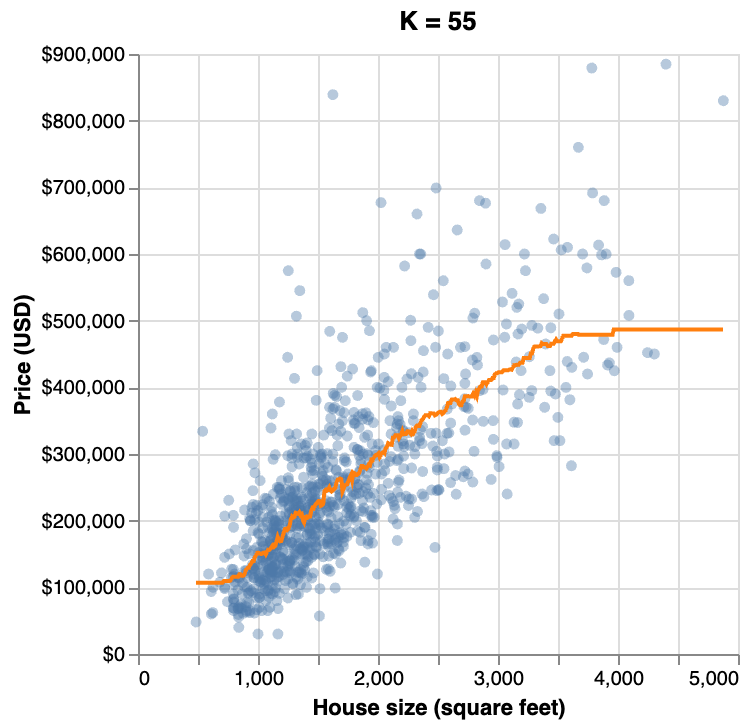
K-NN regression supports multiple predictors - see the end of the slides for Python code demonstrating multivariable K-NN regression.
K-NN regression in scikit-learn
We won’t be covering K-NN regression in detail, as the process is very similar to K-NN classification. The main differences are summarized below:
| Feature | K-NN Classification | K-NN Regression |
|---|---|---|
| Target | Categorical | Continuous |
| Logic | Majority vote | Mean |
| Class | KNeighborsClassifier |
KNeighborsRegressor |
| Output | Label | Value |
| Metrics | Accuracy, Precision, Recall | RMSPE |
Strengths and limitations of K-NN regression
Strengths:
- simple, intuitive algorithm
- requires few assumptions about what the data must look like
- works well with non-linear relationships (i.e., if the relationship is not a straight line)
Weaknesses:
- very slow as the training data gets larger
- may not perform well with a large number of predictors
- may not predict well beyond the range of values input in your training data
Linear Regression
Addresses some of the limitations from KNN regression
Provides an interpretable mathematical equation that describes the relationship between the predictor and response variables
Creates a straight line of best fit through the training data
Note
Logistic regression is the linear model we can use for binary classification
Sacramento real estate
Sacramento real estate: best fit line
The equation for the line is:
\[\text{house price} = \beta_0 + \beta_1 \cdot (\text{house size})+\varepsilon,\] where
- \(\beta_0\) is the vertical intercept of the line (the price when house size is 0)
- \(\beta_1\) is the slope of the line (how quickly the price increases as you increase house size)
- \(\varepsilon\) is the random error term
Sacramento real estate: Prediction
Estimating a line
What makes the best line?
To define the best line we need to know how to measure the distance of the points to the line!
Which of the following criteria would you choose to define “distance of a point to the line”?
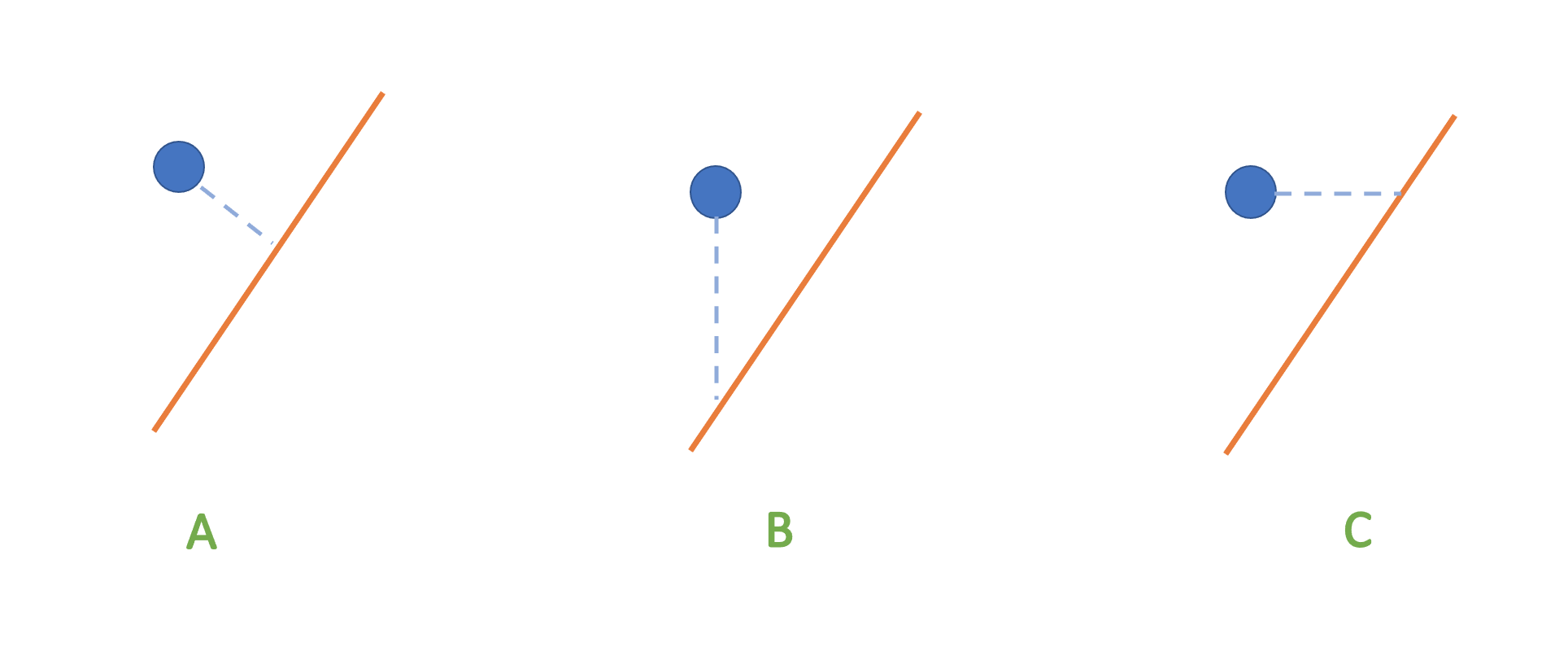
Figure by Dr. Joel Ostblom
Least squares
Least Squares method minimizes the sum of the squares of the residuals. The residuals are the difference between the observed value of the response (\(y_i\)) and the predicted value of the response (\(\hat{y}_i\)):
\[r_i = y_i-\hat{y}_i\]
The residuals are the vertical distances of each point to the estimated line
Sum of squared errors
When estimating the regression equation, we minimize the sum of squared errors (SSE), defined as
\[SSE = \sum_{i=1}^n (y_i-\hat{y_i})^2=\sum_{i=1}^n r_i^2.\]
Linear regression in Python
The scikit-learn pattern still applies:
- Create a training and test set
- Instantiate a model
- Fit the model on training
- Use model on testing set
Linear regression: Train test split
Linear regression: Fit the model
\(\text{house sale price} =\) 15642.31 + 137.29 \(\cdot (\text{house size}).\)
where:
Intercept (\(\hat{\beta}_0=15642.31\)): Predicted sale price when house size = 0 (not meaningful in reality, but needed for the equation).
House size (\(\hat{\beta}_1=137.29\)): Each extra unit of size (e.g., square foot) increases the price by $137.29 on average.
Linear regression: Predictions
Linear regression: Plot
Standarization
- We did not need to standarize like we did for KNN.
- In linear regression, if we standarize, we convert all the units to unit-less standard deviations
- Standarization in linear regression does not change the fit of the model
- It will, however, change the coefficients!
Multiple linear regression
- More predictor variables! (More does not always mean better…)
- When \(p\), the number of variables, is greater than 1, we have multiple linear regression.
Note: We will talk about categorical predictors later in the workshop
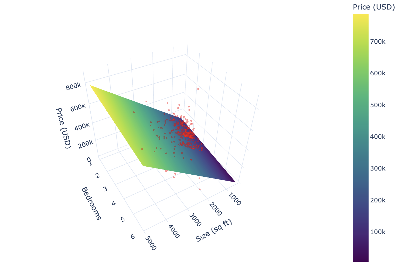
Sacramento real estate: 2 predictors
Sacramento real estate: Coefficients
\[\text{house sale price} = 53180.27 + 154.59\cdot(\text{house size}) -20333.43\cdot(\text{bedrooms}),\] where:
Intercept (\(\hat{\beta}_0=53180.27\)): Predicted sale price when house size = 0 and bedrooms = 0 (not meaningful in reality, but needed for the equation).
House size (\(\hat{\beta}_1=154.59\)): Holding bedrooms constant, each extra unit of size (e.g., square foot) increases the price by $154.59 on average.
Number of bedrooms (\(\hat{\beta}_2=-20333.43\)): Holding size constant, each additional bedroom reduces price by about $20,333.
More variables make it harder to visualize
Sacramento real estate: mlm rmspe
Outliers and Multicollinearity
- Outliers: extreme values that can move the best fit line
- Multicollinearity: variables that are highly correlated to one another
Outliers
Subset
Full data
Multicollinearity
Multicollinearity means that some (or all) of the explanatory variables are linearly related!
When this happens, the coefficient estimates are very “unstable” and the contribution of one variable gets mixed with that of another variable correlated with it.
Essentially, the plane of best fit has regression coefficients that are very sensitive to the exact values in the data.
Feature selection
- In modern datasets, we often have many features (sometimes more than the number of observations).
- Not all features are informative or relevant.
- Including irrelevant predictors can lead to:
- Overfitting
- Multicollinearity
- Poor generalization to new data
- We need methods that can automatically select features while fitting the model…
L1-regularization
- L1-regularization, often referred to as LASSO (Least Absolute Shrinkage and Selection Operator), adds an L1 penalty to the least squares loss:
\[ \hat{\boldsymbol{\beta}} = \arg\min_{\boldsymbol{\beta}} \left\{ \sum_{i=1}^n (y_i - \mathbf{x}_i^\top \boldsymbol{\beta})^2 + \lambda \sum_{j=1}^p |\beta_j| \right\} \]
- \(\lambda \geq 0\) is a tuning parameter that controls the strength of the penalty
- With the L1 penalty, many coefficients get set equal to zero.
- Thus, LASSO performs variable selection and regularization.
Note
Standardization is necessary in penalized regression because penalty terms are scale-sensitive.
L1-regularization in scikit-learn
Choosing the shrinkage parameter
- The \(\alpha\) parameter controls the strength of the L1 penalty:
- Larger \(\alpha\) → stronger regularization → more coefficients shrunk to zero
- Smaller \(\alpha\) → less regularization → more complex model
- Proper selection of \(\alpha\) is critical for balancing bias and variance.
Tuning \(\alpha\) with cross-validation
Just like tuning \(k\) in KNN, we can select \(\alpha\) by evaluating performance on validation sets.
Example workflow with GridSearchCV:
Knowledge check
Alternatively, go to menti.com and use code 1668 5101
Additional Resources
- The Regression I: K-nearest neighbors and Regression II: linear regression chapters of Data Science: A First Introduction (Python Edition) by Tiffany Timbers, Trevor Campbell, Melissa Lee, Joel Ostblom, Lindsey Heagy contains all the content presented here with a detailed narrative.
- The
scikit-learnwebsite is an excellent reference for more details on, and advanced usage of, the functions and packages in this lesson. Aside from that, it also offers many useful tutorials to get you started. - An Introduction to Statistical Learning by Gareth James Daniela Witten Trevor Hastie, and Robert Tibshirani provides a great next stop in the process of learning about classification. Chapter 3 discusses lienar regression in more depth. As well as how it comares to K-nearest neighbors.
References
Thomas Cover and Peter Hart. Nearest neighbor pattern classification. IEEE Transactions on Information Theory, 13(1):21–27, 1967.
Evelyn Fix and Joseph Hodges. Discriminatory analysis. nonparametric discrimination: consistency properties. Technical Report, USAF School of Aviation Medicine, Randolph Field, Texas, 1951.
Code for CV in K-NN regression
Multivariable K-NN regression: Preprocessor
Multivariable K-NN regression: CV
Multivariable K-NN regression: Best K
Multivariable K-NN regression: Best model
Best K
Best RMSPE