Ink & Paper
- Complete themes
- Geom element
- Use in layers
Complete themes
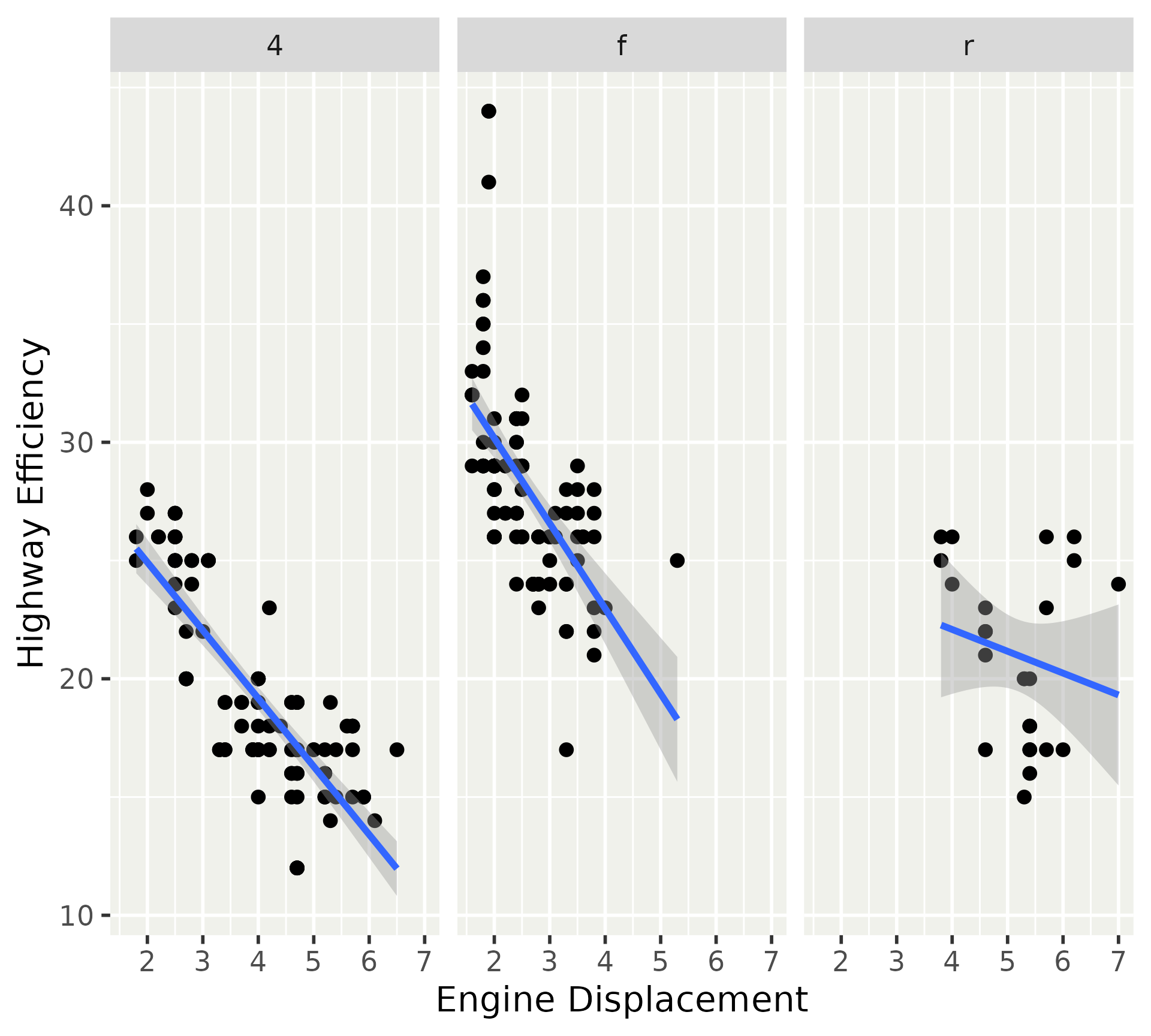
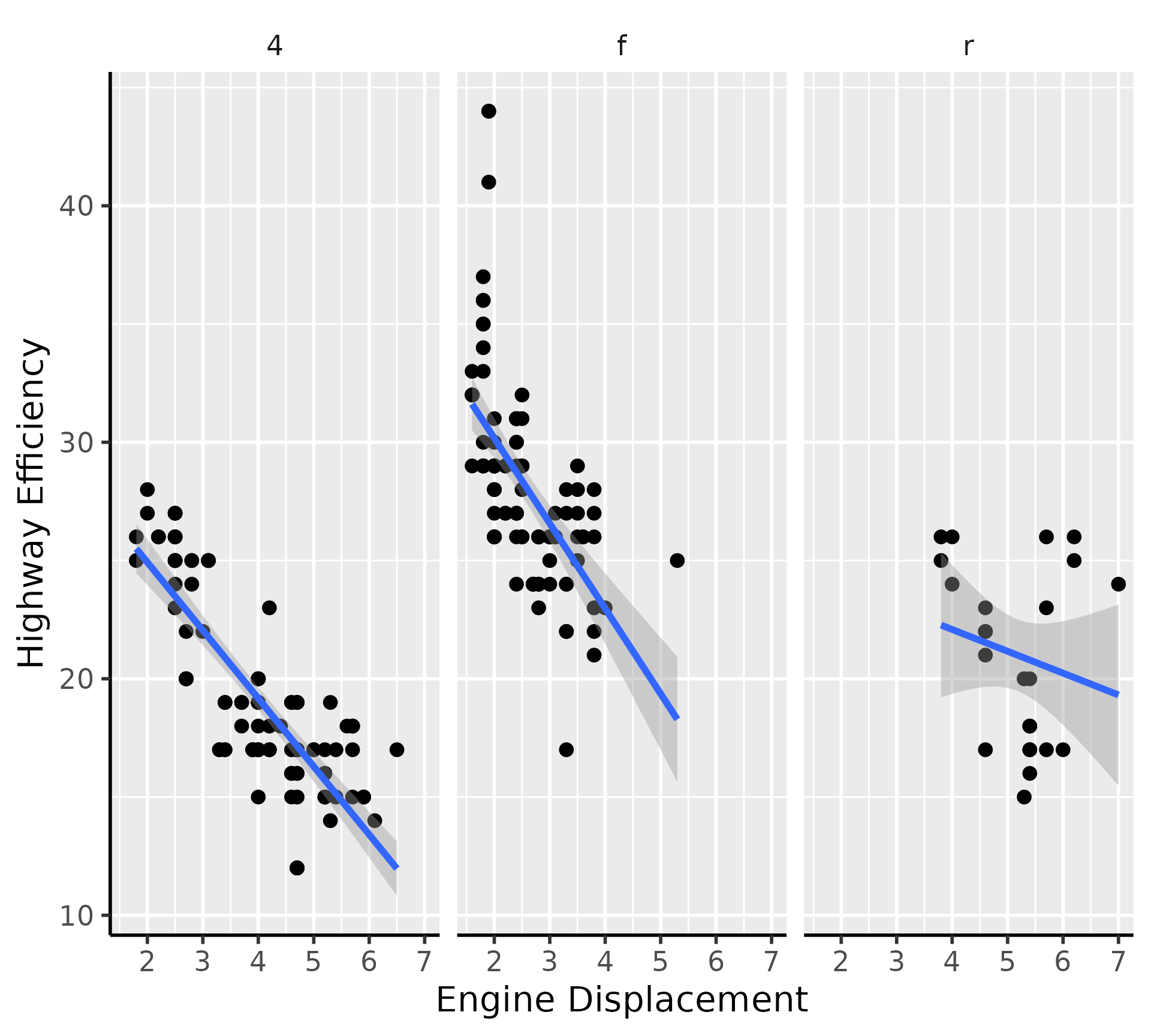
library(ggplot2)

p <- ggplot(mpg) +
  aes(displ, hwy) +
  geom_point() +
  geom_smooth(
    aes(displ, hwy),
    formula = y ~ x, method = "lm",
    inherit.aes = FALSE
  ) +
  facet_wrap(~ drv) +
  labs(dictionary = c(
      cty = "City\nEfficiency",
      hwy = "Highway Efficiency",
      displ = "Engine Displacement",
      year = "Year",
      "factor(year)" = "Year",
      class = "Class"
  ))
p
Complete themes
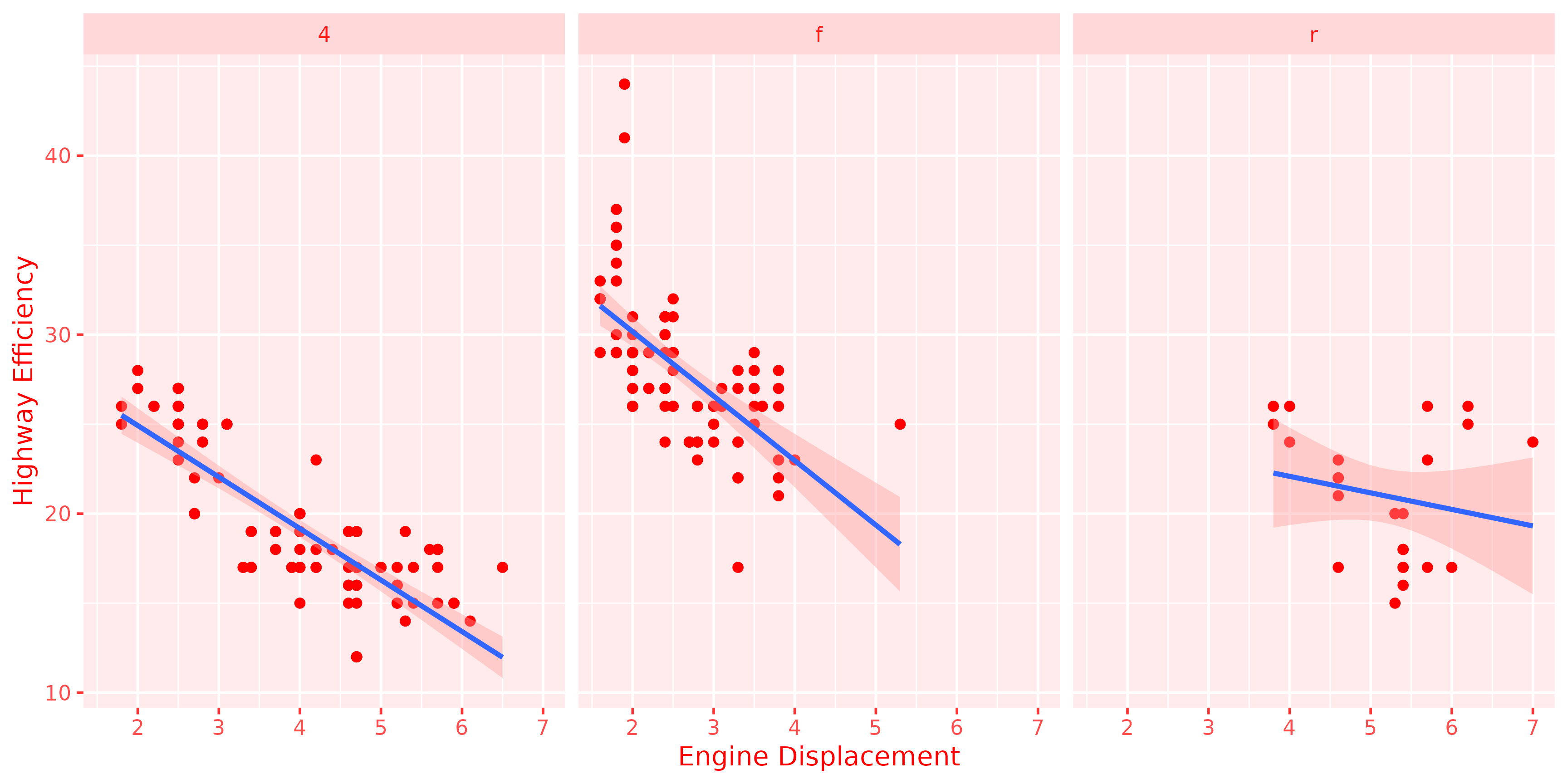
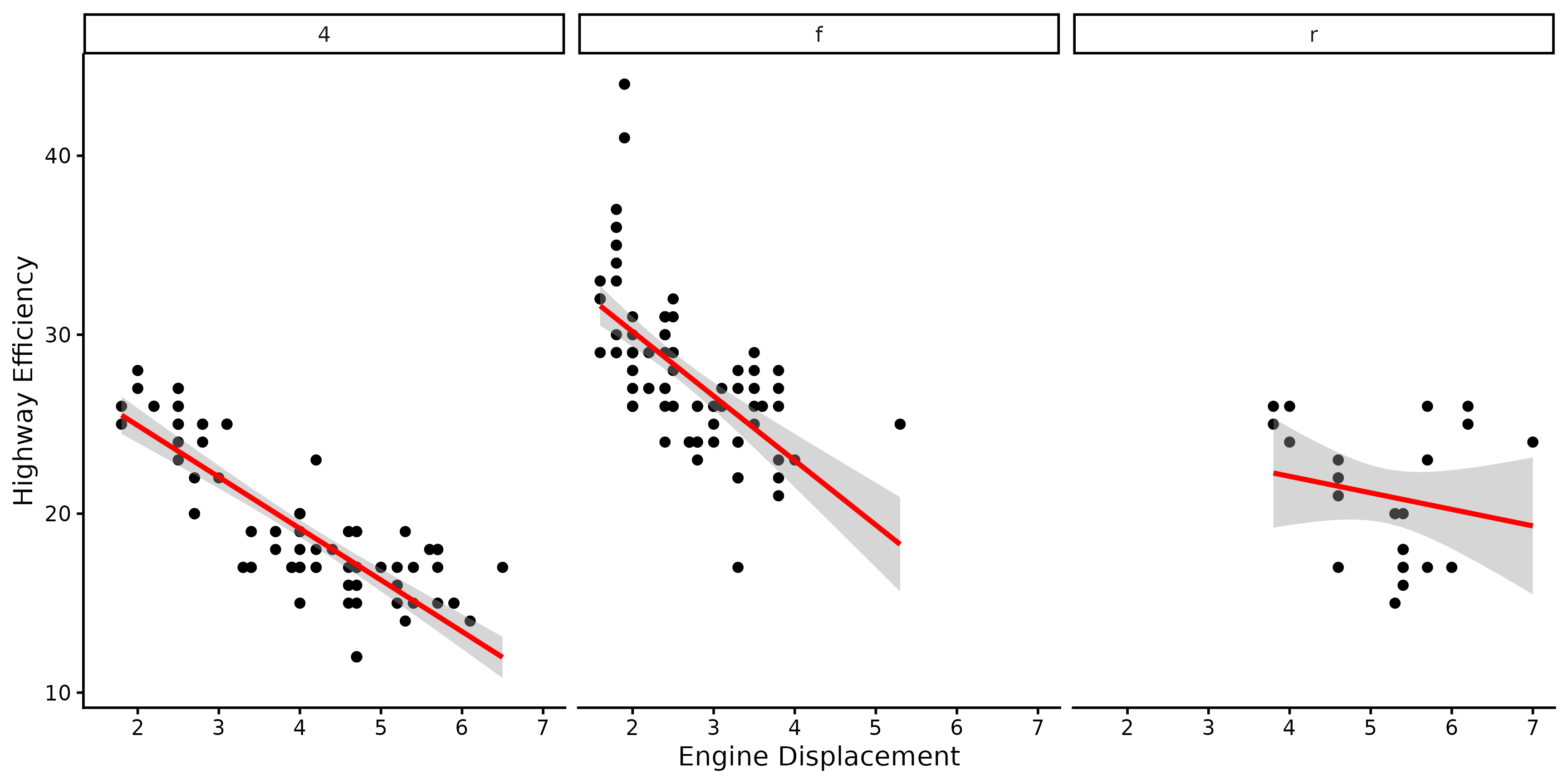
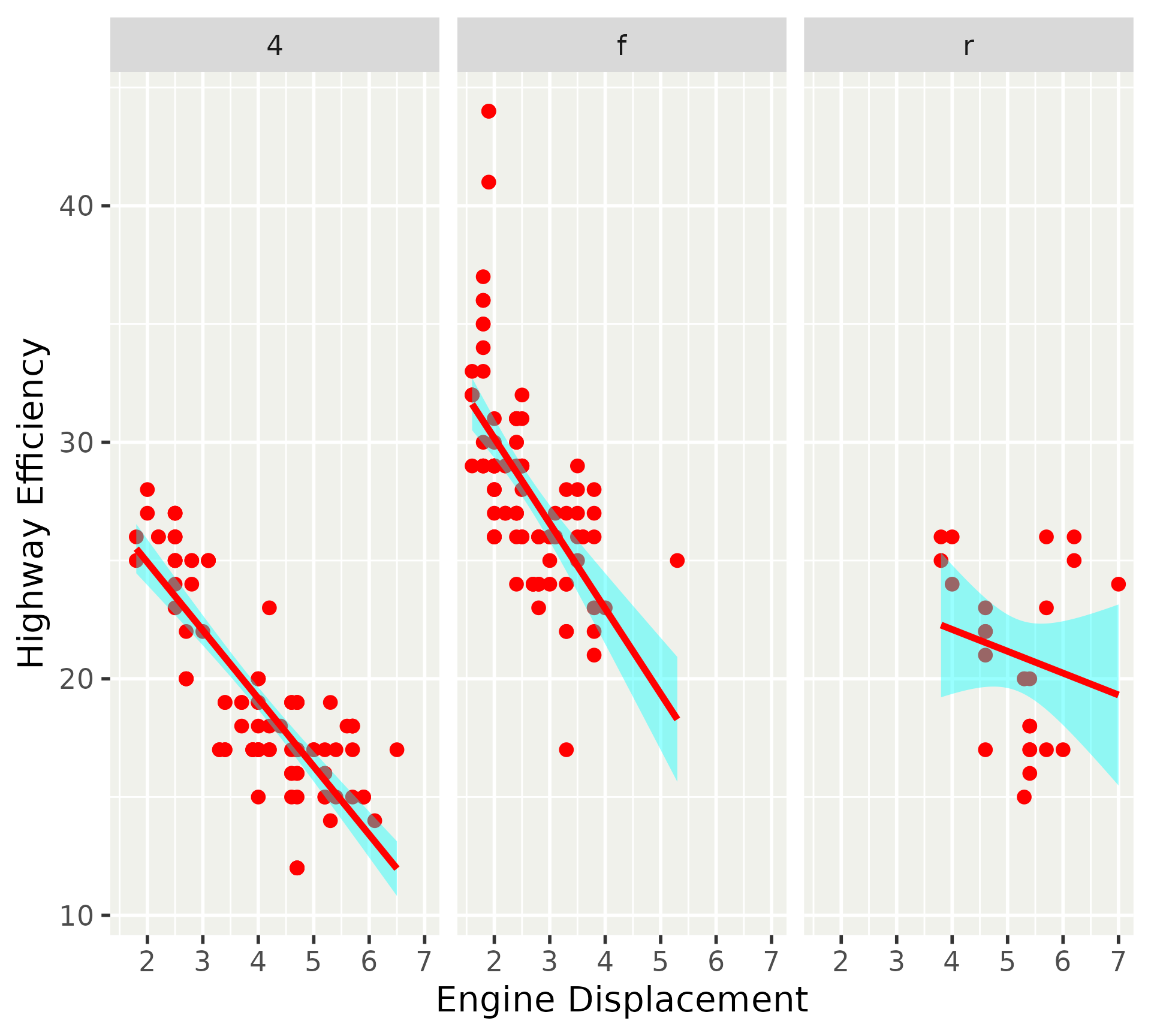
ink affects all foreground elements and parts of layers.
p + theme_gray(ink = "red")
![]()
Complete themes
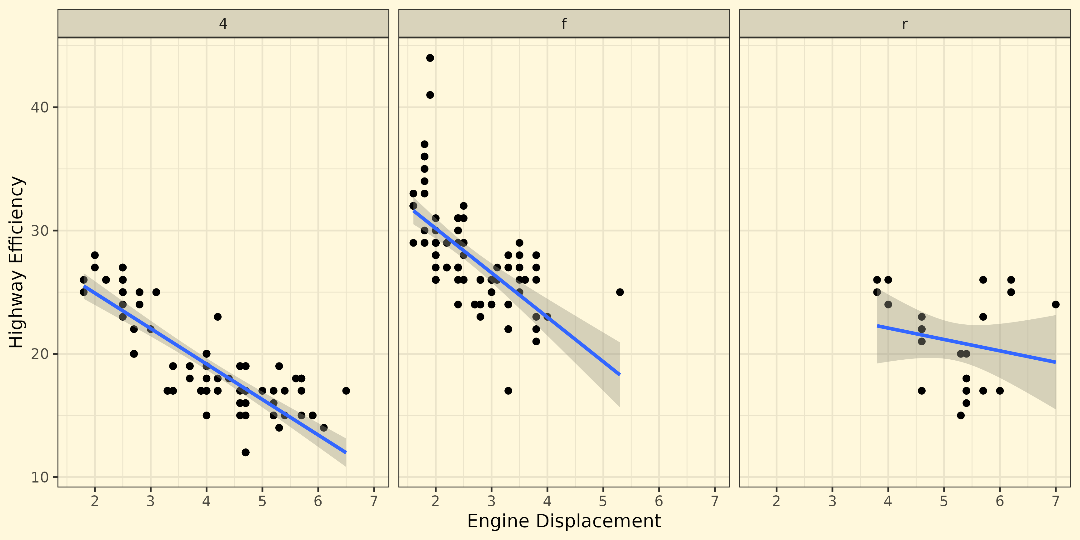
paper affects all background elements and parts of layers.
p + theme_bw(paper = "cornsilk")
![]()
Complete themes
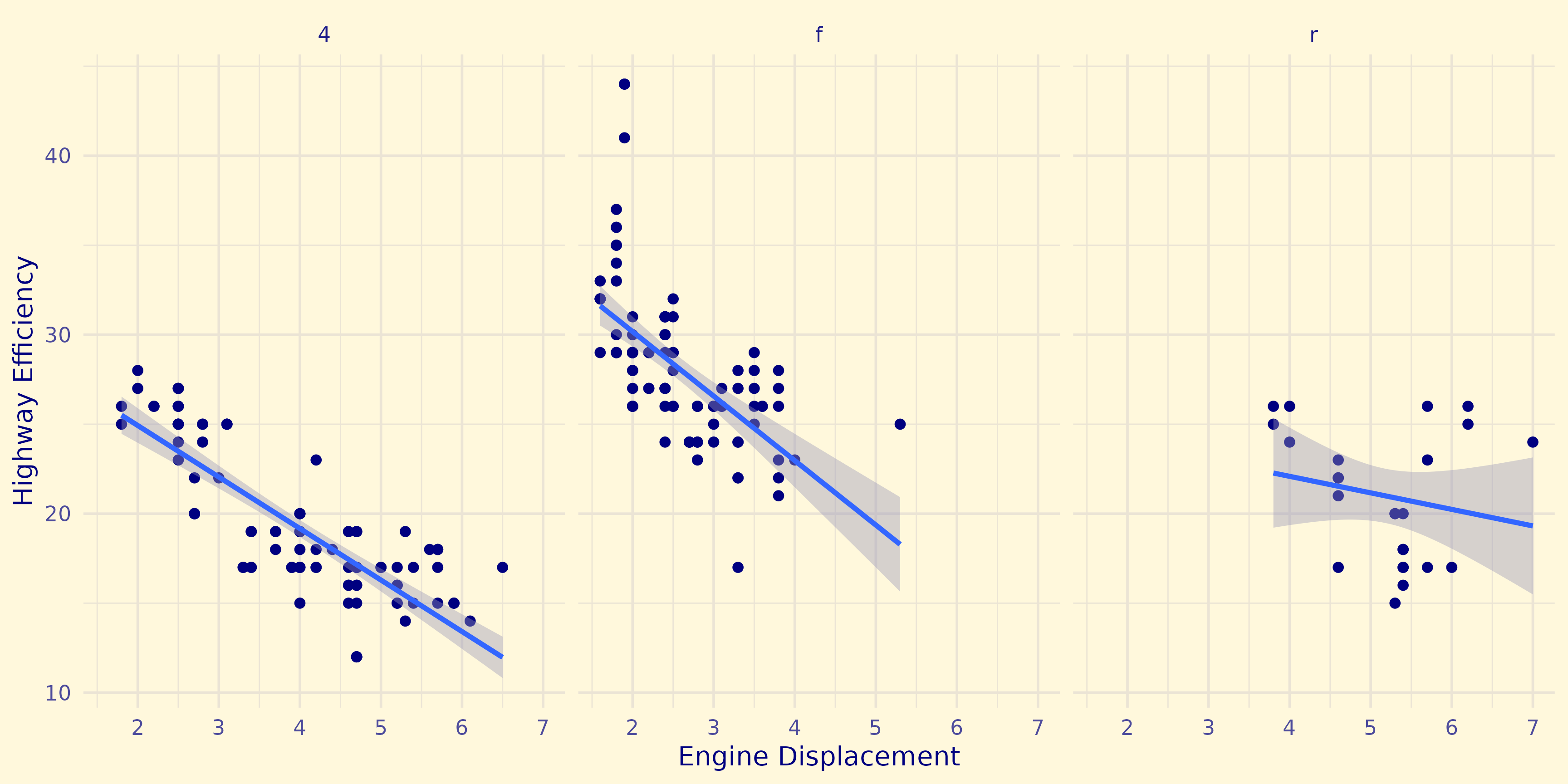
ink and paper can be combined to recolour a plot.
p + theme_minimal(paper = "cornsilk", ink = "navy")
![]()
Complete themes
accent has niche application in geom_smooth() and geom_contour().
p + theme_classic(accent = "red")
![]()
Geom elements
theme(geom) accommodates the layer settings
p + theme(geom = element_geom(
  ink    = "red",
  accent = "black"
))
Geom elements
ink/paper/accent act as described for complete themes
element_geom()
## <ggplot2::element_geom>
##  @ ink        : NULL
##  @ paper      : NULL
##  @ accent     : NULL
##  @ linewidth  : NULL
##  @ borderwidth: NULL
##  @ linetype   : NULL
##  @ bordertype : NULL
##  @ family     : NULL
##  @ fontsize   : NULL
##  @ pointsize  : NULL
##  @ pointshape : NULL
##  @ colour     : NULL
##  @ fill       : NULL
Geom elements
For lines, we distinguish borders (of polygons) and ‘naked’ lines.
element_geom()
## <ggplot2::element_geom>
##  @ ink        : NULL
##  @ paper      : NULL
##  @ accent     : NULL
##  @ linewidth  : NULL
##  @ borderwidth: NULL
##  @ linetype   : NULL
##  @ bordertype : NULL
##  @ family     : NULL
##  @ fontsize   : NULL
##  @ pointsize  : NULL
##  @ pointshape : NULL
##  @ colour     : NULL
##  @ fill       : NULL
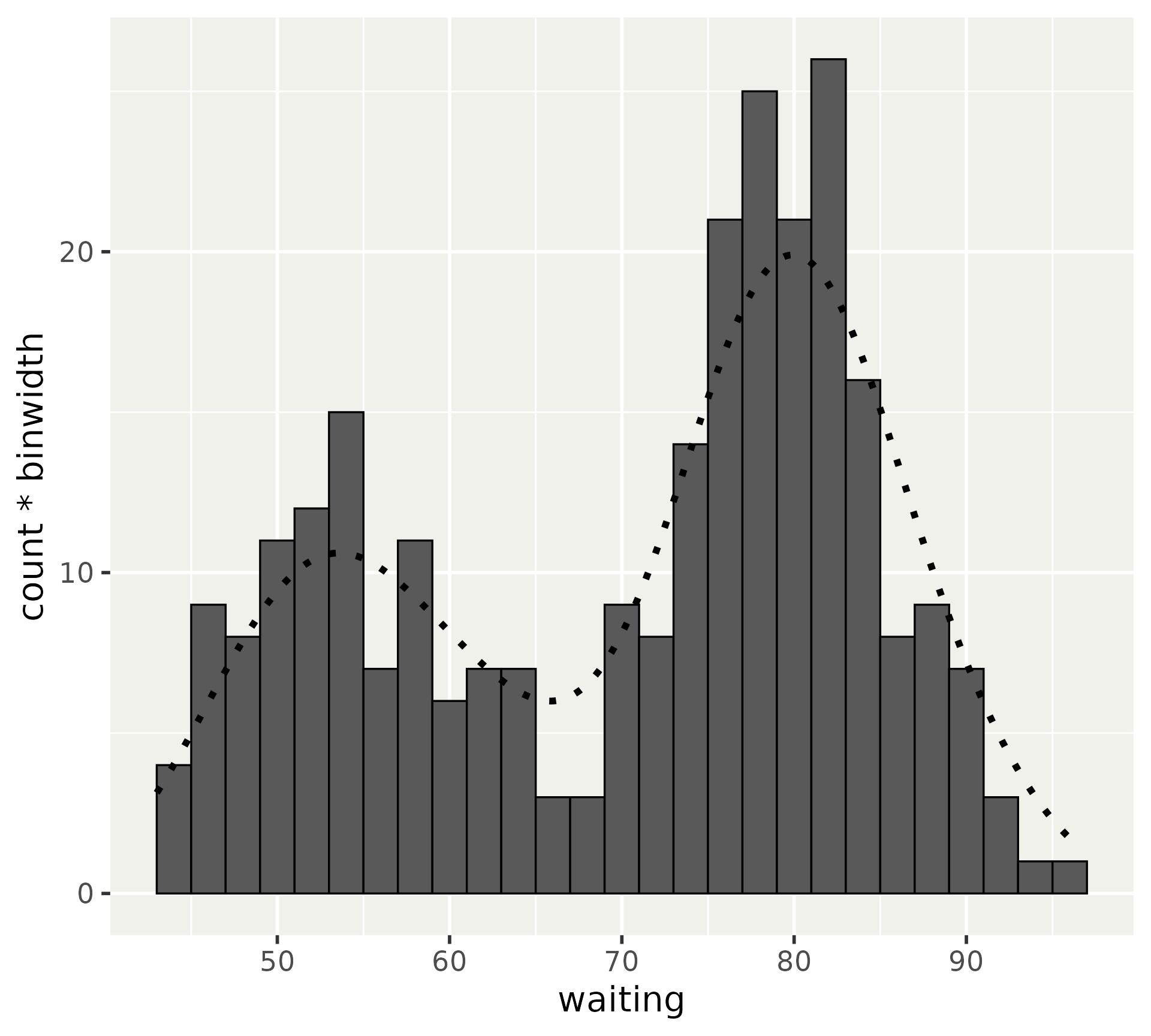
Geom elements
Illustration of polygon border versus naked line
binwidth <- 2
ggplot(faithful, aes(waiting)) +
  geom_histogram(
    colour = "black", binwidth = binwidth
  ) +
  geom_density(
    aes(y = after_stat(count * binwidth))
  ) +
  theme(geom = element_geom(
    # Affects histogram
    borderwidth = 0.3,
    bordertype  = "solid",
    # Affects density line
    linewidth = 1,
    linetype  = "dotted"
  ))
Geom elements
For text, we can set family and fontsize
element_geom()
## <ggplot2::element_geom>
##  @ ink        : NULL
##  @ paper      : NULL
##  @ accent     : NULL
##  @ linewidth  : NULL
##  @ borderwidth: NULL
##  @ linetype   : NULL
##  @ bordertype : NULL
##  @ family     : NULL
##  @ fontsize   : NULL
##  @ pointsize  : NULL
##  @ pointshape : NULL
##  @ colour     : NULL
##  @ fill       : NULL
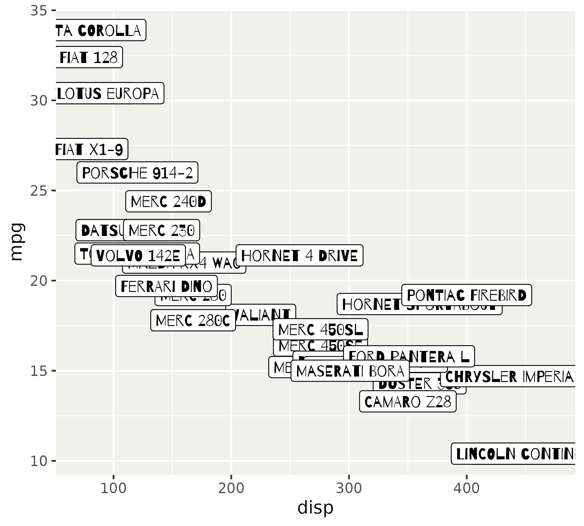
Geom elements
For text, we can set family and fontsize
ggplot(mtcars) +
  aes(disp, mpg, label = rownames(mtcars)) +
  geom_label() +
  theme(
    geom = element_geom(
      family = "Barrio",
      fontsize = 10
    )
  )
Geom elements
For points, we can set pointsize and pointshape
element_geom()
## <ggplot2::element_geom>
##  @ ink        : NULL
##  @ paper      : NULL
##  @ accent     : NULL
##  @ linewidth  : NULL
##  @ borderwidth: NULL
##  @ linetype   : NULL
##  @ bordertype : NULL
##  @ family     : NULL
##  @ fontsize   : NULL
##  @ pointsize  : NULL
##  @ pointshape : NULL
##  @ colour     : NULL
##  @ fill       : NULL
Geom elements
For points, we can set pointsize and pointshape
p + theme(geom = element_geom(
  pointsize  = 2,
  pointshape = "triangle"
))
Geom elements
There is also the familiar colour and fill.
element_geom()
## <ggplot2::element_geom>
##  @ ink        : NULL
##  @ paper      : NULL
##  @ accent     : NULL
##  @ linewidth  : NULL
##  @ borderwidth: NULL
##  @ linetype   : NULL
##  @ bordertype : NULL
##  @ family     : NULL
##  @ fontsize   : NULL
##  @ pointsize  : NULL
##  @ pointshape : NULL
##  @ colour     : NULL
##  @ fill       : NULL
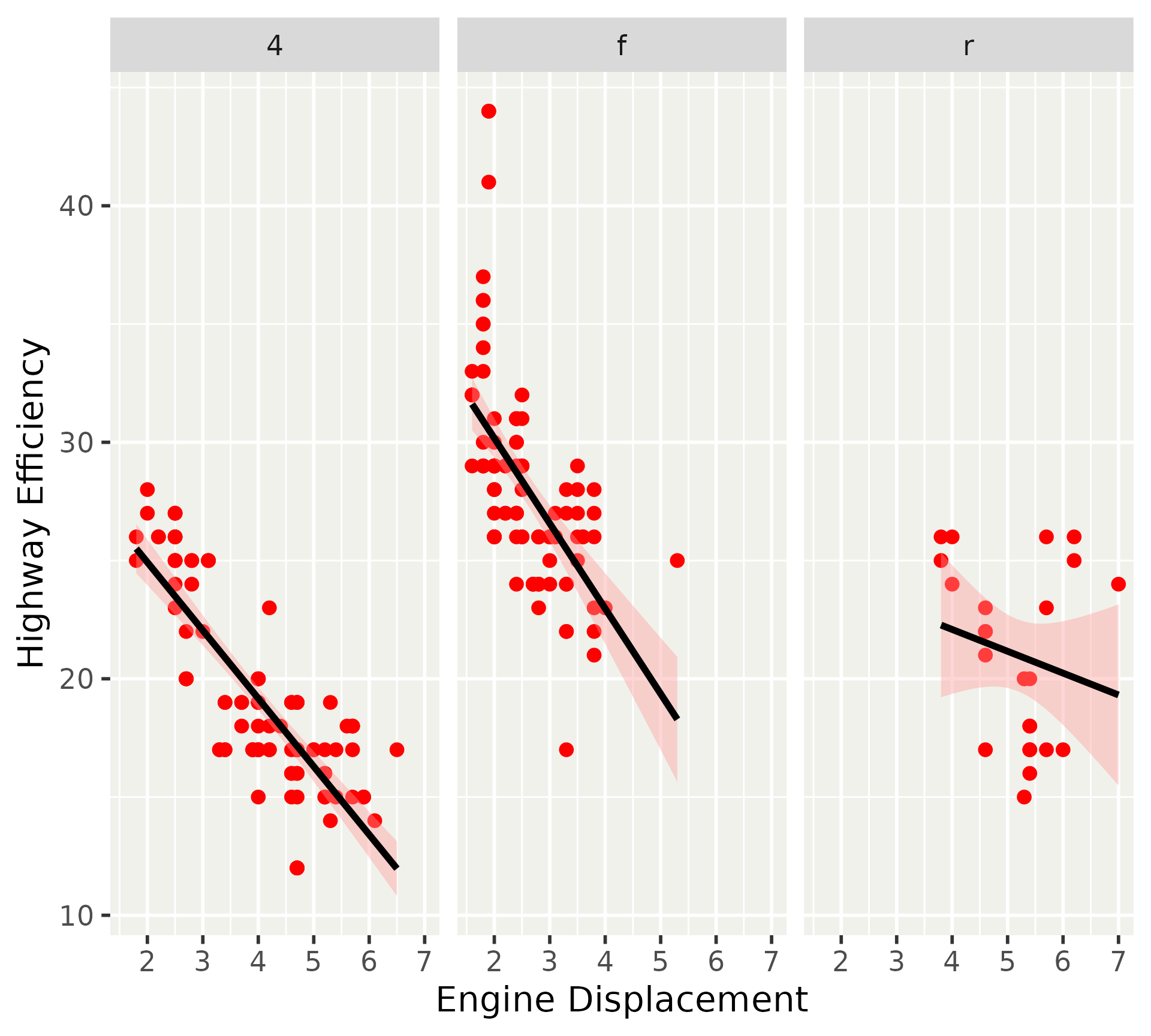
Geom elements
colour and fill are direct, but indiscriminate. Note how accent is now ignored.
p + theme(geom = element_geom(
  colour = "red",
  fill   = "cyan",
  accent = "limegreen"
))
Geom elements
colour and fill are designed to tailor for individual geom types.
p + theme(
  geom.point  = element_geom(colour = "dodgerblue"),
  geom.smooth = element_geom(colour = "navy")
)
Ink & Paper: summary
- Complete themes can be used to coordinate a colour scheme quickly.
theme_complete(ink, paper, accent)
- Most layer defaults can be set in the theme.
theme(geom = element_geom(...))
Default palettes
Several ways to set a plot’s colour palette
- Directly add a scale
+ scale_colour_gradientn()- Not set as default scale
- Using esoteric options
options(ggplot2.continuous.colour = scale_colour_gradientn)- Arcane
- Overriding default scale
scale_colour_continuous <- scale_colour_gradientn- Messes with namespace
- NEW: via
theme()
Controlling palettes
A tour through various options
my_palette <- hcl.colors(15, "sunset")
custom_scale <- function(...) {
scale_colour_gradientn(colours = my_palette, ...)
}
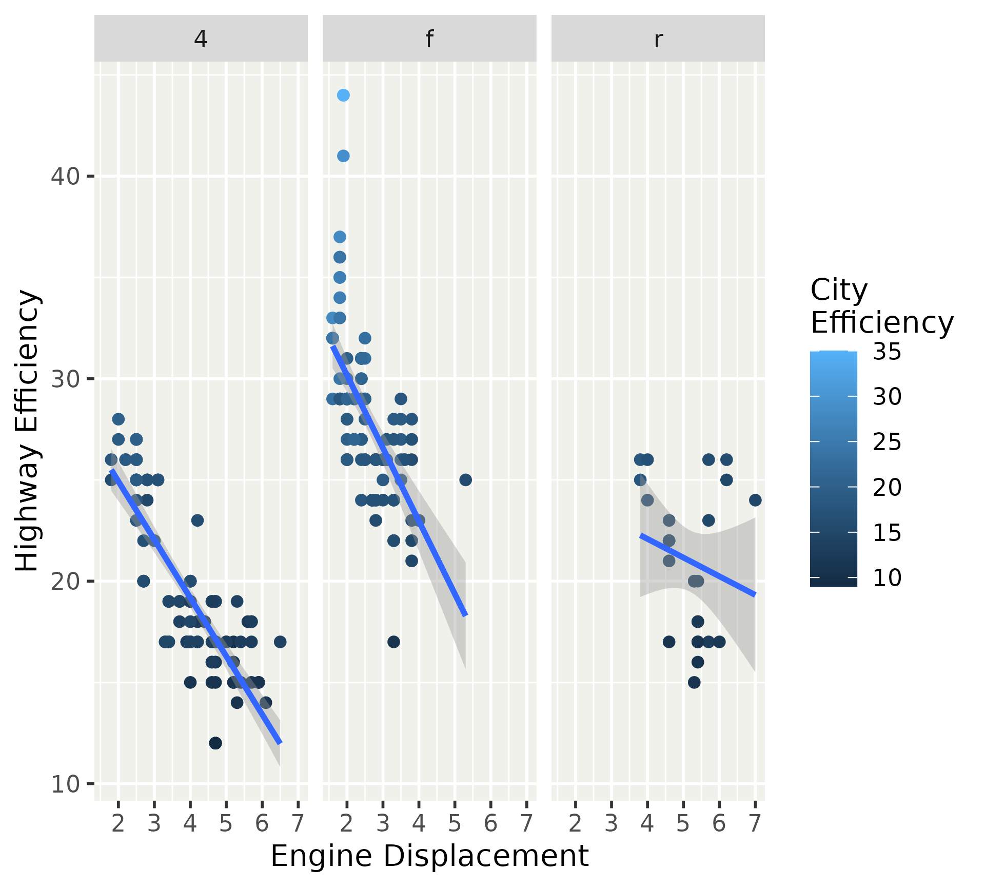
p2 <- p + aes(colour = cty)
# 1. Directly set a scale
p2 + scale_colour_gradientn(colors = my_palette)
# 2. Using options
options(ggplot2.continuous.colour = custom_scale)
p2
options(ggplot2.continuous.colour = NULL) # reset
# 3. Redefine scale
scale_colour_continuous <- custom_scale
p2
scale_colour_continuous <- ggplot2::scale_colour_continuous # reset
# 4. Using theme
p2 + theme(palette.colour.continuous = my_palette)
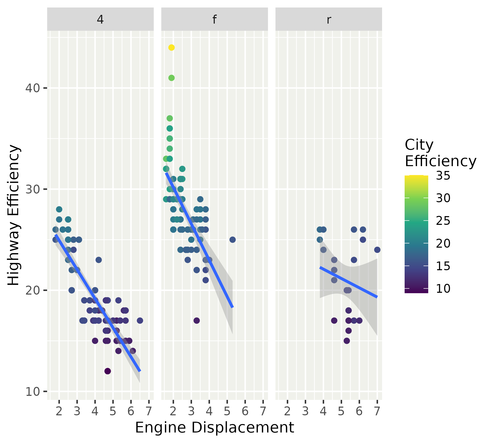
Controlling palettes
Regular scales override theme defaults
p2 +
  theme(palette.colour.continuous = my_palette) +
  scale_colour_viridis_c()
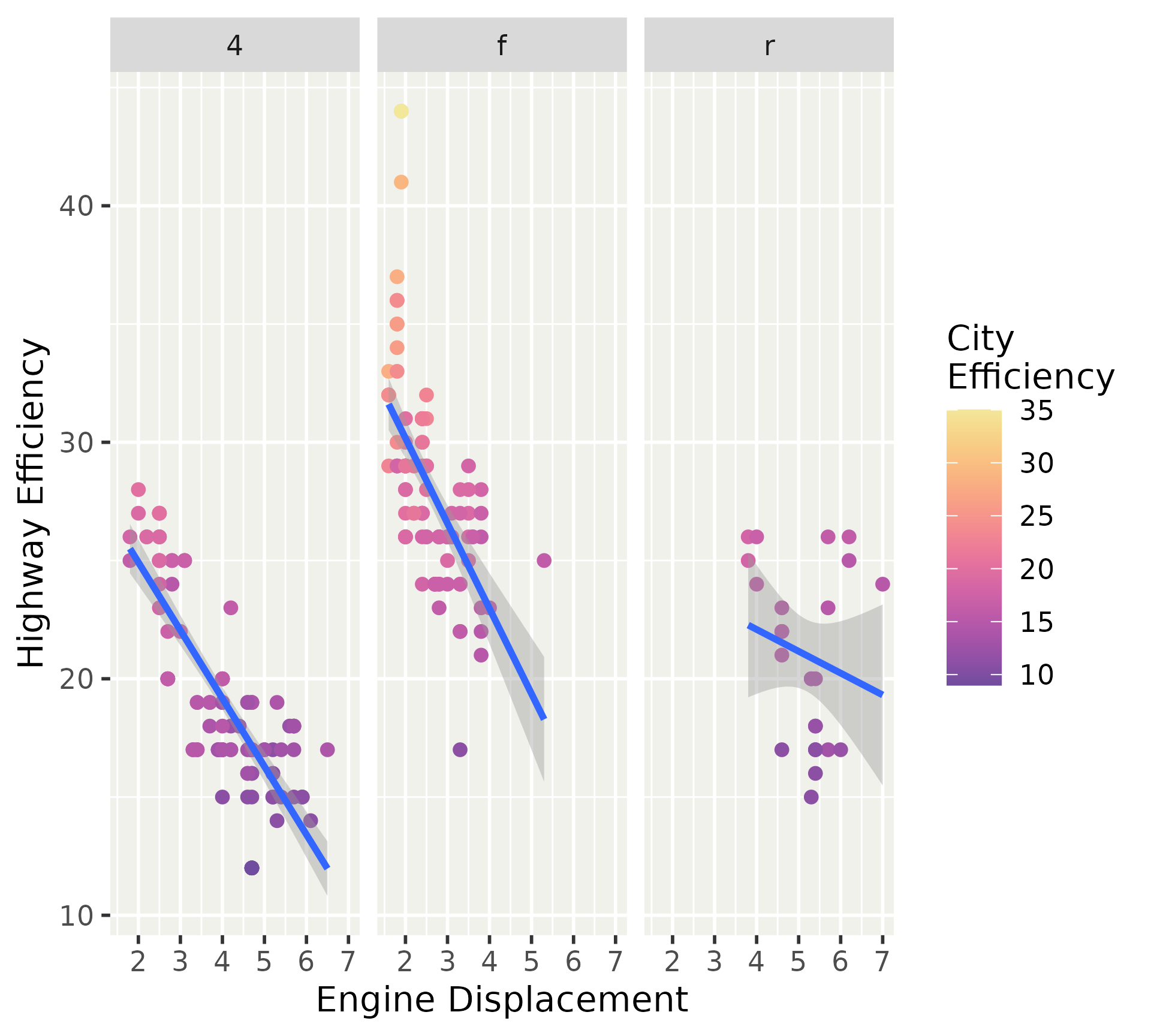
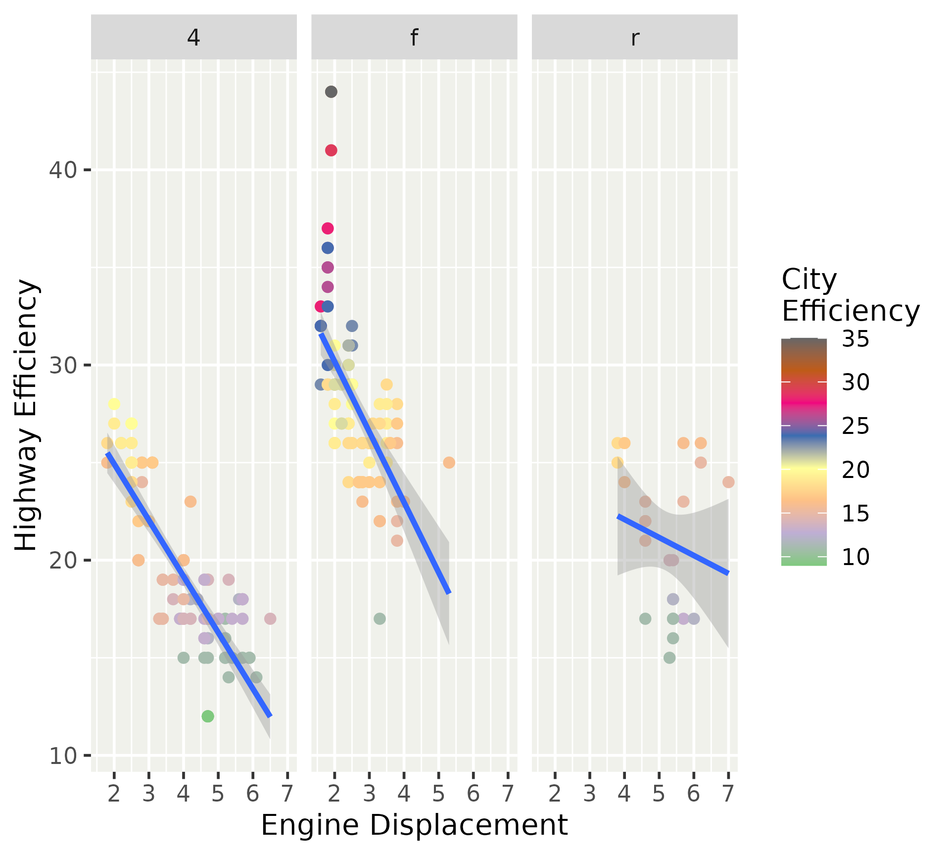
Controlling palettes
The default palette does not commit to a full scale. You can still tweak the options via the default scales (scale_{aesthetic}_{type}).
p2 +
  theme(palette.colour.continuous = my_palette) +
  scale_colour_continuous(
    breaks = c(
      ten    = 10,
      twenty = 20,
      thirty = 30
    )
  )
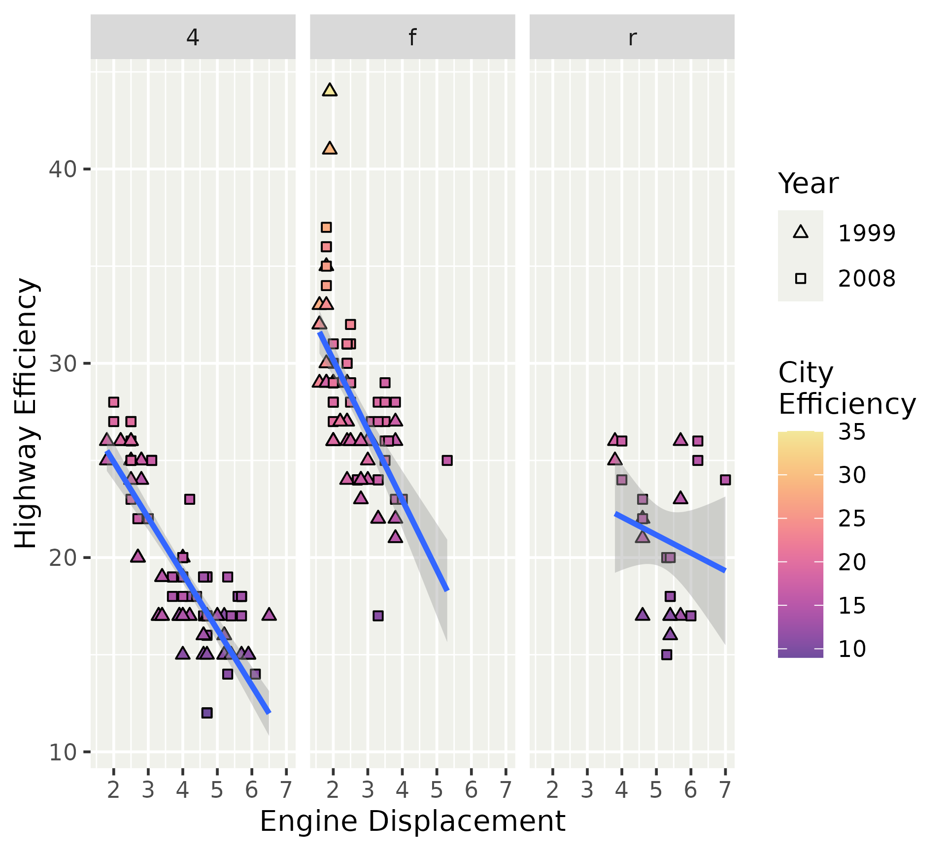
Theme palettes
The palette settings have the syntax palette.{aesthetic}.{type}, where type can be "continuous" or "discrete".
shapes <- c("triangle filled", "square filled")
p +
  aes(
    fill = cty,
    shape = factor(year)
  ) +
  theme(
    palette.shape.discrete = shapes,
    palette.fill.continuous = "sunset"
  )
The palatable palettes are those that can pass through scales::as_continuous_pal() and scales::as_discrete_pal() respectively.
library(scales)
# Discrete palettes
pal <- as_discrete_pal(c("foo", "bar", "qux"))
pal(2)
## [1] "foo" "bar"
palette_type(pal)
## [1] "character"
palette_nlevels(pal)
## [1] 3
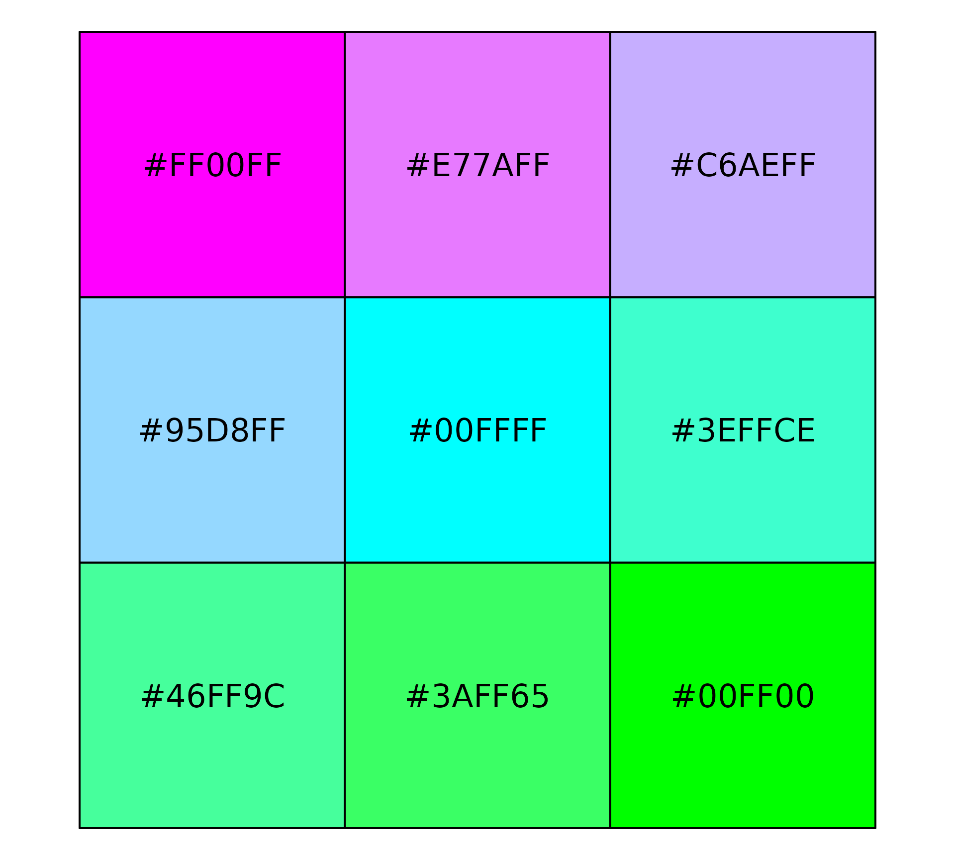
# Colours as continuous palette
pal <- as_continuous_pal(c("magenta", "green"))
pal(c(0, 0.5, 1))
## [1] "#FF00FF" "#C9B2A2" "#00FF00"
palette_type(pal)
## [1] "colour"
With the right metadata, we can interchange discrete and continuous palettes.
pal <- new_discrete_palette(
  pal_manual(c("magenta", "cyan", "green")),
  type = "colour", nlevels = 3
)

is_continuous_pal(pal)
## [1] FALSE

con_pal <- as_continuous_pal(pal)
is_continuous_pal(con_pal)
## [1] TRUE

seq(0, 1, length.out = 9) |>
  con_pal() |>
  show_col()
Just because we can swap discrete and continuous palettes, doesn’t mean we should!
p2 + theme(
  # No! What have I done?!
  palette.colour.continuous = pal_brewer("qual")
)
Default palettes: summary
- New theme arguments to set default palettes:
palette.{aes}.{type}.
- Input for discrete palettes
scales::as_discrete_palette().
- Input for continuous palettes
scales::as_continuous_palette().
Build your own theme
How do you intend to use a personal theme?
- Complete theme
- Partial theme
Building a complete theme
Capture your theme as a function.
my_theme <- function(...) {
  NULL
}

p + my_theme()
Building a complete theme
Start with using a complete theme as base.
my_theme <- function(...) {
  theme_gray(...)
}

p + my_theme()
Building a complete theme
Build your own customisations on top.
my_theme <- function(...) {
  theme_gray(...) +
    theme(
      axis.line = element_line(),
      strip.background = element_blank()
    )
}

p + my_theme()
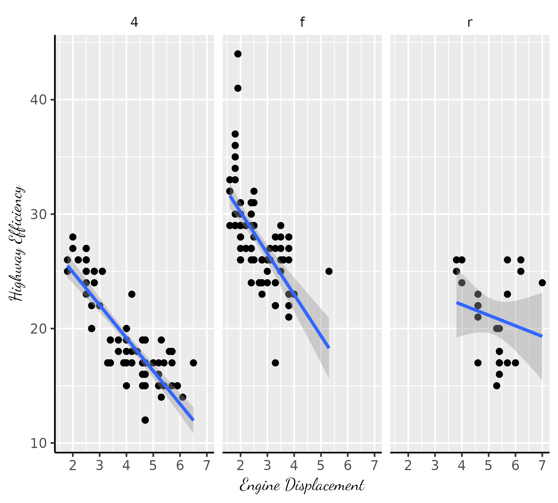
Building a complete theme
For custom fonts, put in guardrails for their possible absence.
my_theme <- function(..., header_family = "Dancing Script") {
  systemfonts::require_font(header_family)
  theme_gray(..., header_family = header_family) +
    theme(
      axis.line = element_line(),
      strip.background = element_blank()
    )
}

p + my_theme()
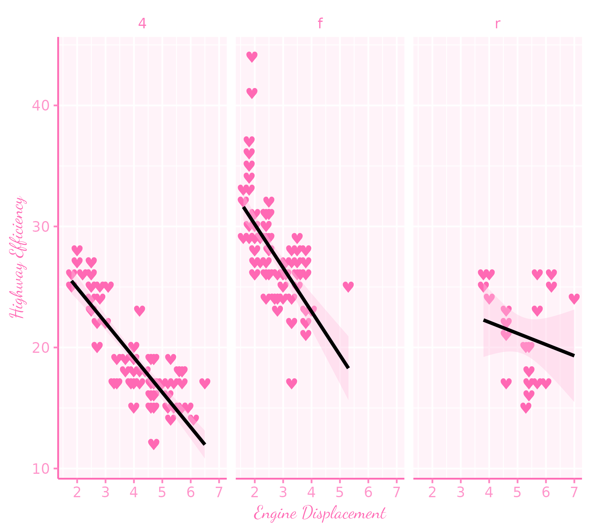
Building a complete theme
You can coordinate the ink/paper/accent settings, along with the geom argument.
my_theme <- function(
  ...,
  ink = "hotpink",
  accent = "black",
  header_family = "Dancing Script"
) {
  systemfonts::require_font(header_family)
  theme_gray(..., ink = ink, accent = accent, header_family = header_family) +
    theme(
      geom = element_geom(pointshape = "♥", pointsize = 3),
      axis.line = element_line(),
      strip.background = element_blank()
    )
}

p + my_theme()
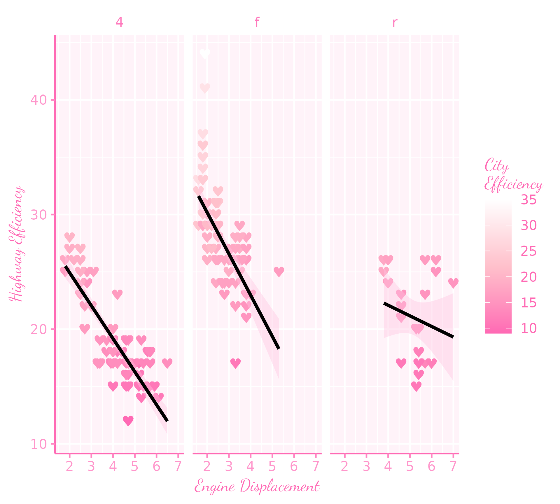
Building a complete theme
If you have flamboyant ink or paper colours, you may also want to direct the palette.colour.continuous and palette.colour.discrete palettes.
my_theme <- function(
  ...,
  ink = "hotpink",
  accent = "black",
  header_family = "Dancing Script"
) {
  systemfonts::require_font(header_family)
  theme_gray(..., ink = ink, accent = accent, header_family = header_family) +
    theme(
      geom = element_geom(pointshape = "♥", pointsize = 3),
      axis.line = element_line(),
      strip.background = element_blank(),
      palette.colour.continuous = c("hotpink", "pink", "white")
    )
}

p2 + my_theme()
Building a complete theme
You can activate your theme for all plots in your document by using set_theme().
set_theme(my_theme())
# Now all plots will be rendered with your theme
p2
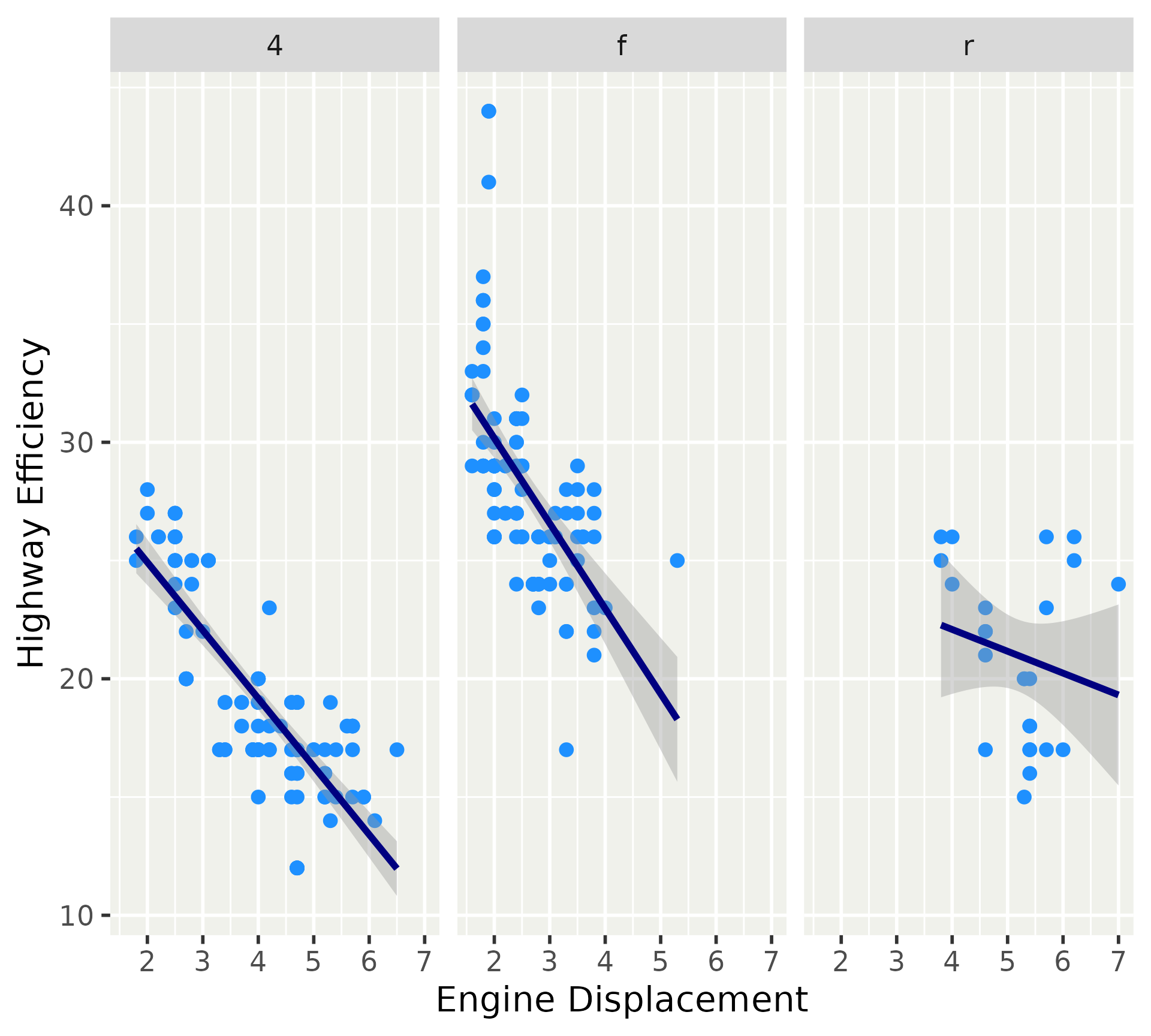
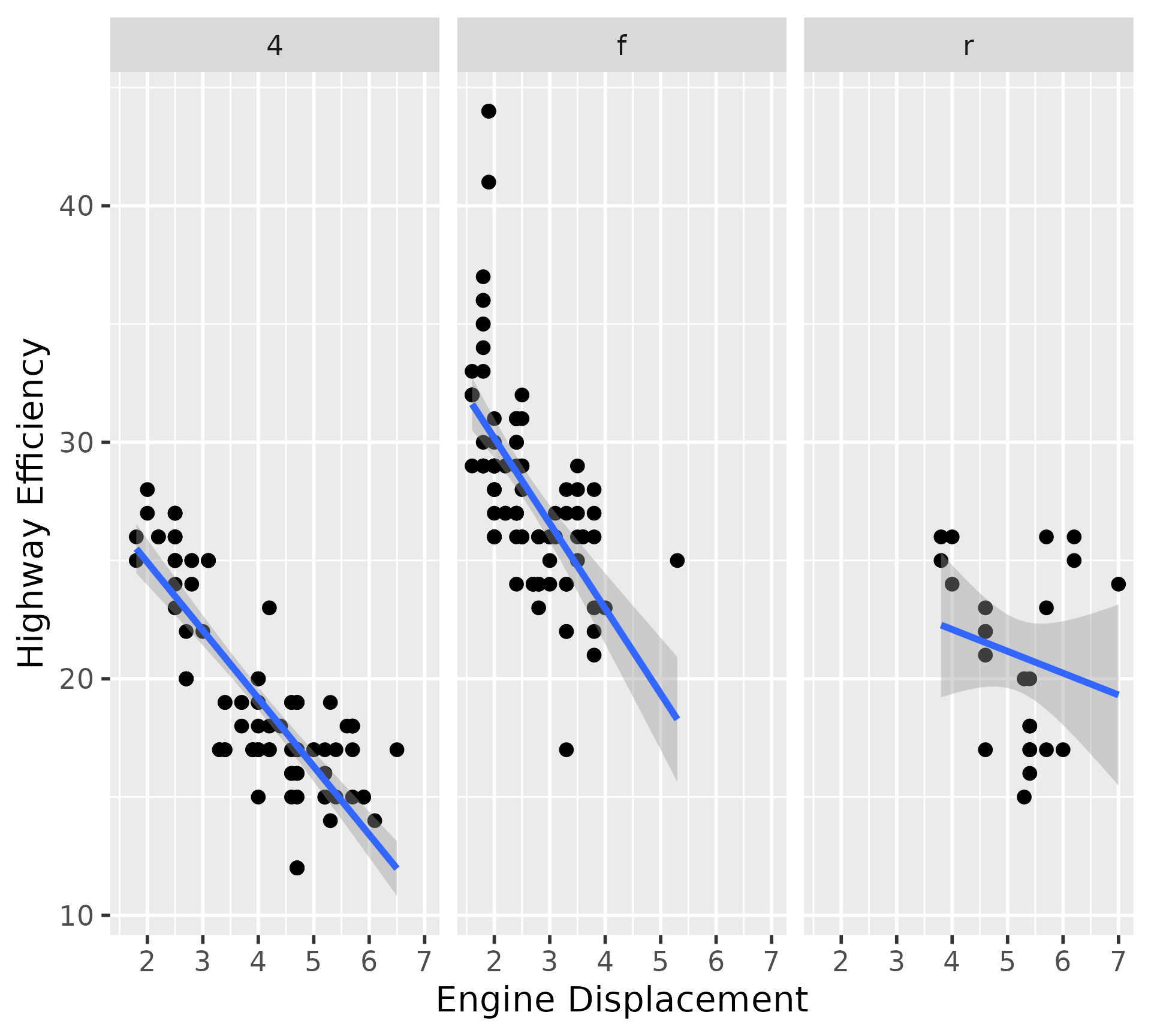
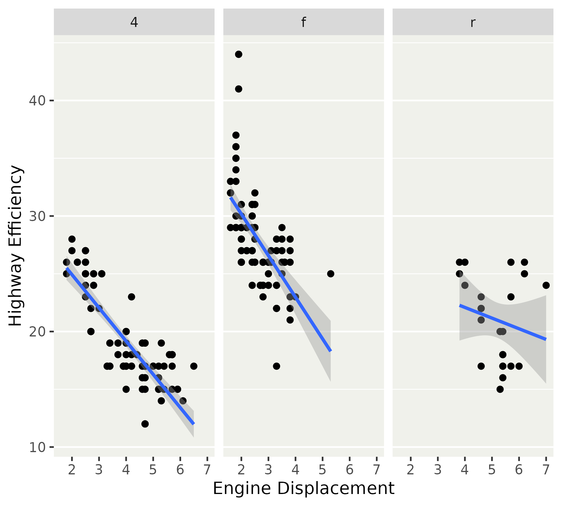
Building a complete theme
But for now, we’ll reset it to something familiar.
set_theme(theme_gray())
p2
![]()
Building a partial theme
For individual plots, the same advice holds for building a theme function.
However, you can have partial theme ‘shortcuts’.
Building a partial theme
You still call a theme() or theme_sub() function to initiate a fresh, (incomplete) theme. No need to start with a complete theme base.
horizontal_grid <- function() {
  theme_sub_panel(
    grid.major.x = element_blank(),
    grid.minor.x = element_blank(),
    grid.major.y = element_line(),
    grid.minor.y = element_line()
  )
}

p + horizontal_grid()
Building your own theme: summary
- Implement as function.
- Use complete theme as basis
- Add on your tweaks
- (Guard custom fonts)
- (Coordinate colour & palettes)
Custom guides
ggplot2 has more guides than colour bars and legends.
- axes
- colour bar
- colour steps
- legend
- binned guide
Base guides
A guide can be specified in guides() or in the scale_*(guide) argument.
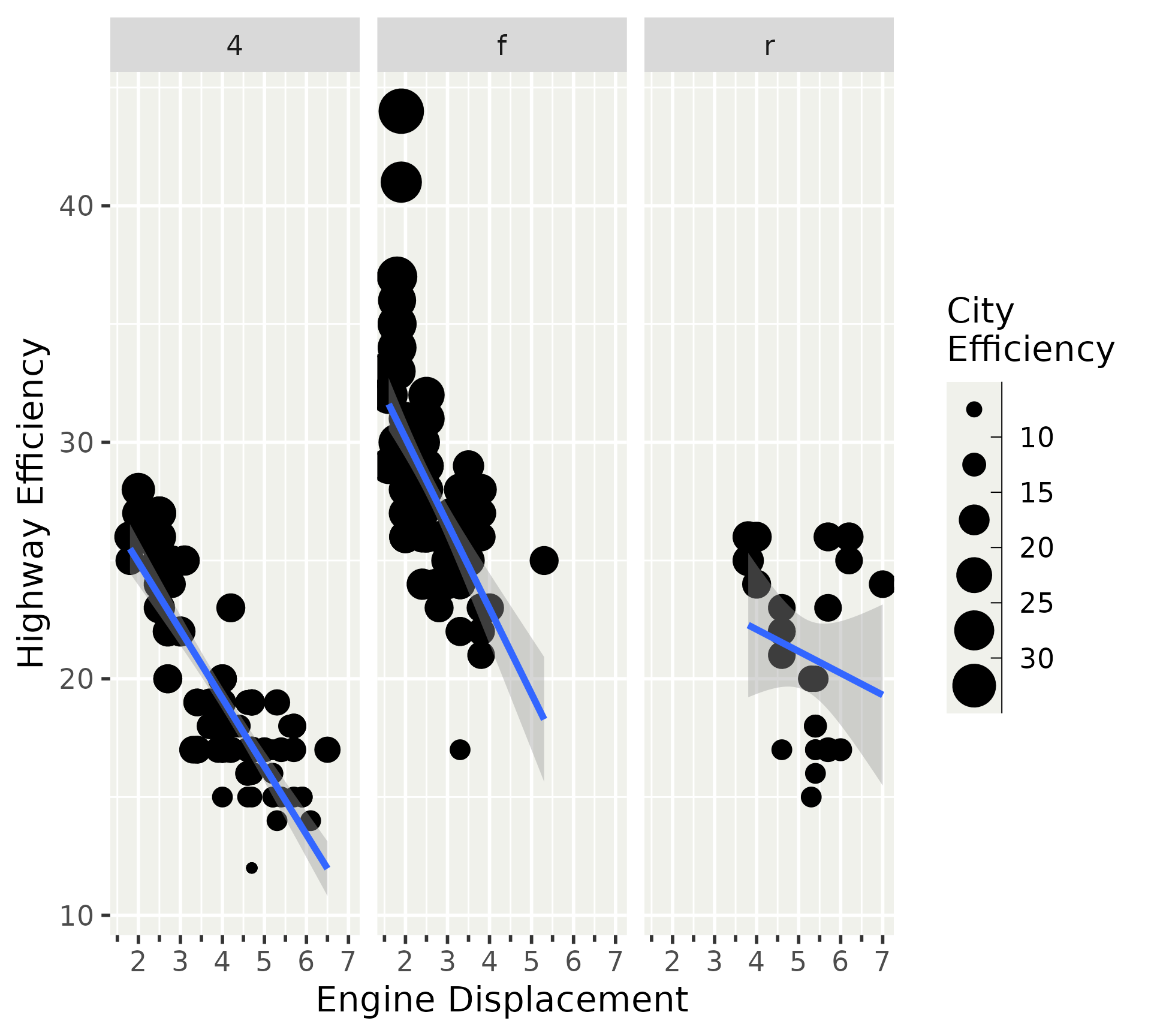
p +
  aes(size = cty) +
  scale_size_continuous(guide = "bins") +
  guides(x = guide_axis(minor.ticks = TRUE))
Styling guides
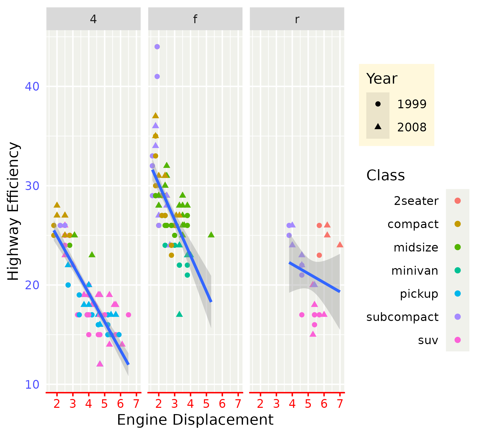
Guides can have their own local themes for customisation.
p +
  aes(shape = factor(year), colour = class) +
  guides(
    x = guide_axis(
      theme = theme_classic(ink = "red")
    ),
    y = guide_axis(
      theme = theme_minimal(ink = "blue")
    ),
    shape = guide_legend(
      theme = theme_gray(paper = "cornsilk")
    ),
    colour = guide_legend(
      theme = theme(legend.text.position = "left")
    )
  )
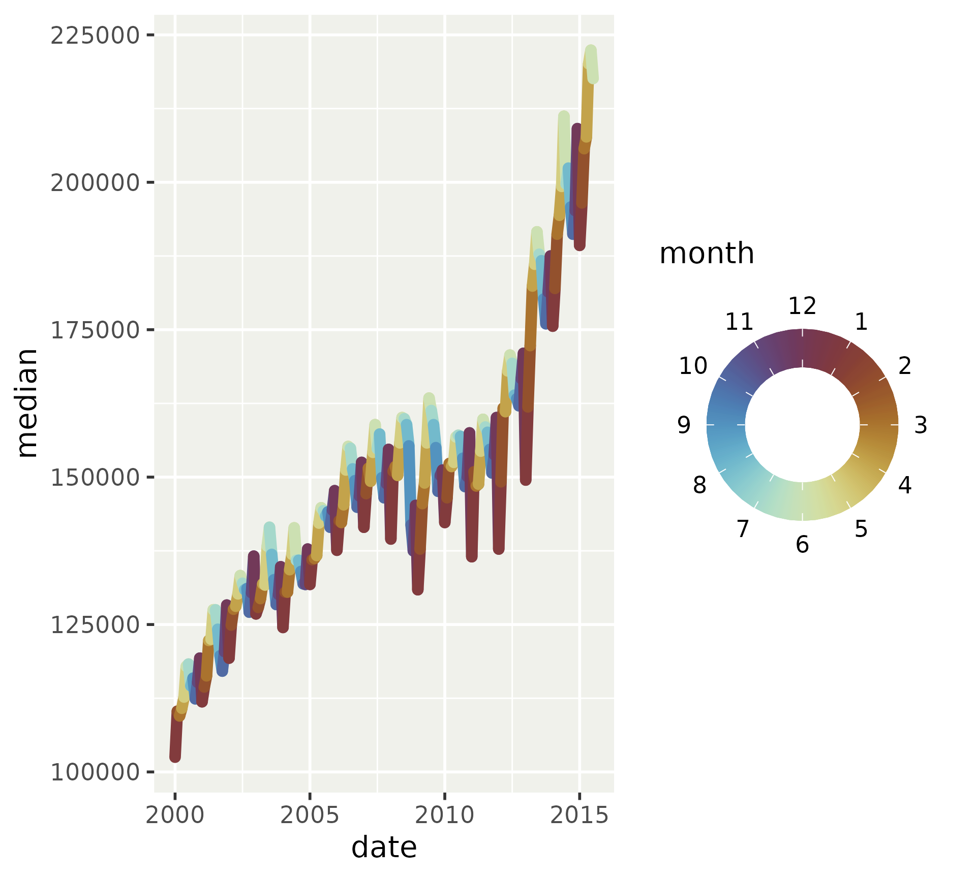
Guide extensions
Specialised guides for niche applications, like periodical data.
library(legendry)

dplyr::filter(txhousing, city == "Houston") |>
  ggplot(aes(date, median, colour = month)) +
  geom_line(linewidth = 2, lineend = "round") +
  scico::scale_colour_scico(
    breaks = 1:12, limits = c(0, 12),
    palette = "romaO",
    guide = "colring"
  ) +
  theme(legend.key.size = unit(5, "mm"))
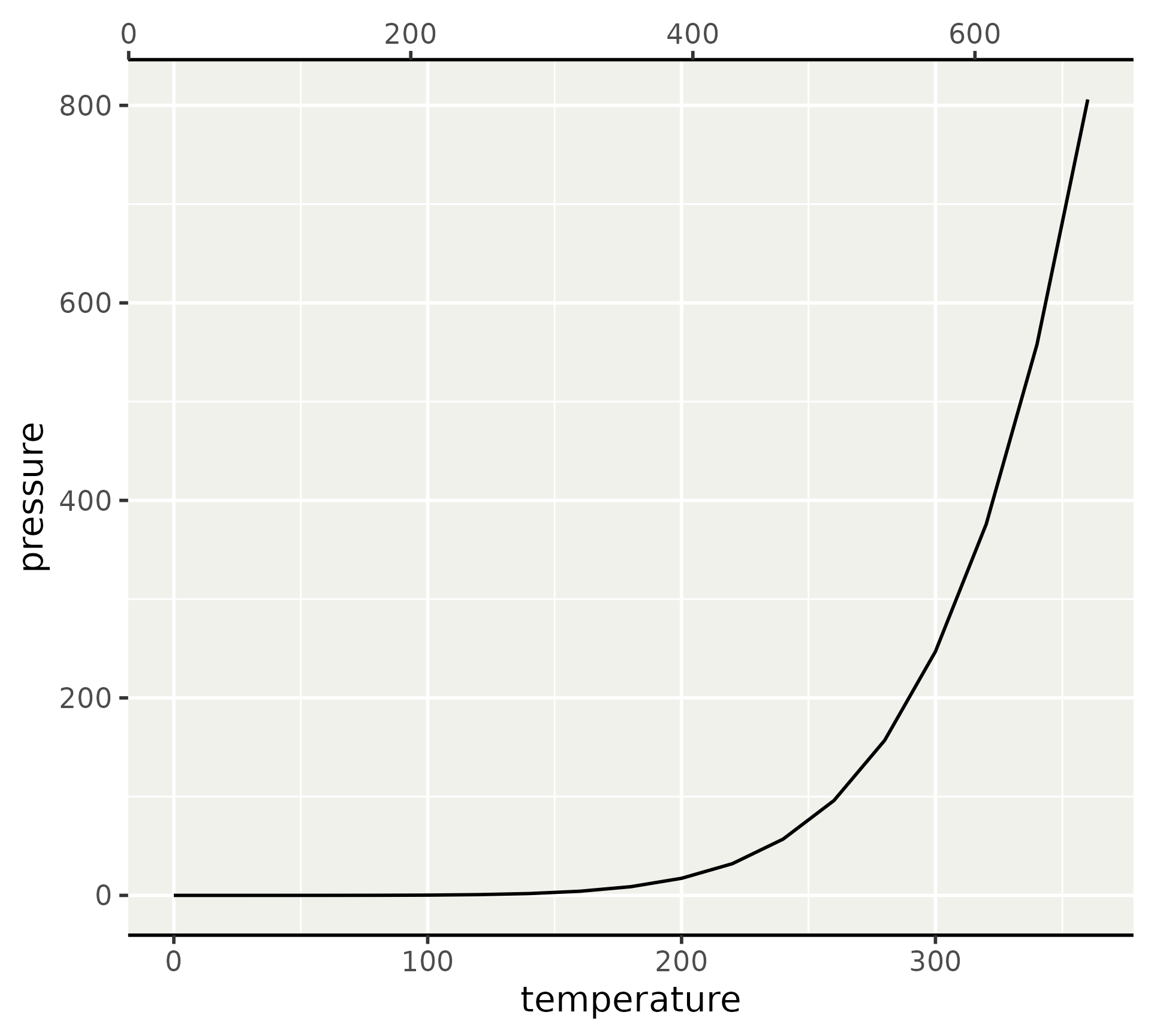
Guide extensions
Guides can be specified flexibly to at least the degree of secondary axes.
# Translate Celsius range to Fahrenheit
deg_C <- range(pressure$temperature)
deg_F <- (deg_C * 9 / 5) + 32
# Compute breaks and translate back to Celsius
deg_F <- scales::extended_breaks()(deg_F)
deg_C <- (deg_F - 32) * 5 / 9

fahrenheit_axis <- guide_axis_base(
  key = key_manual(aesthetic = deg_C, label = deg_F)
)

p3 <- ggplot(pressure) +
  aes(temperature, pressure) +
  geom_line() +
  theme(axis.line.x = element_line())

p3 + guides(x.sec = fahrenheit_axis)
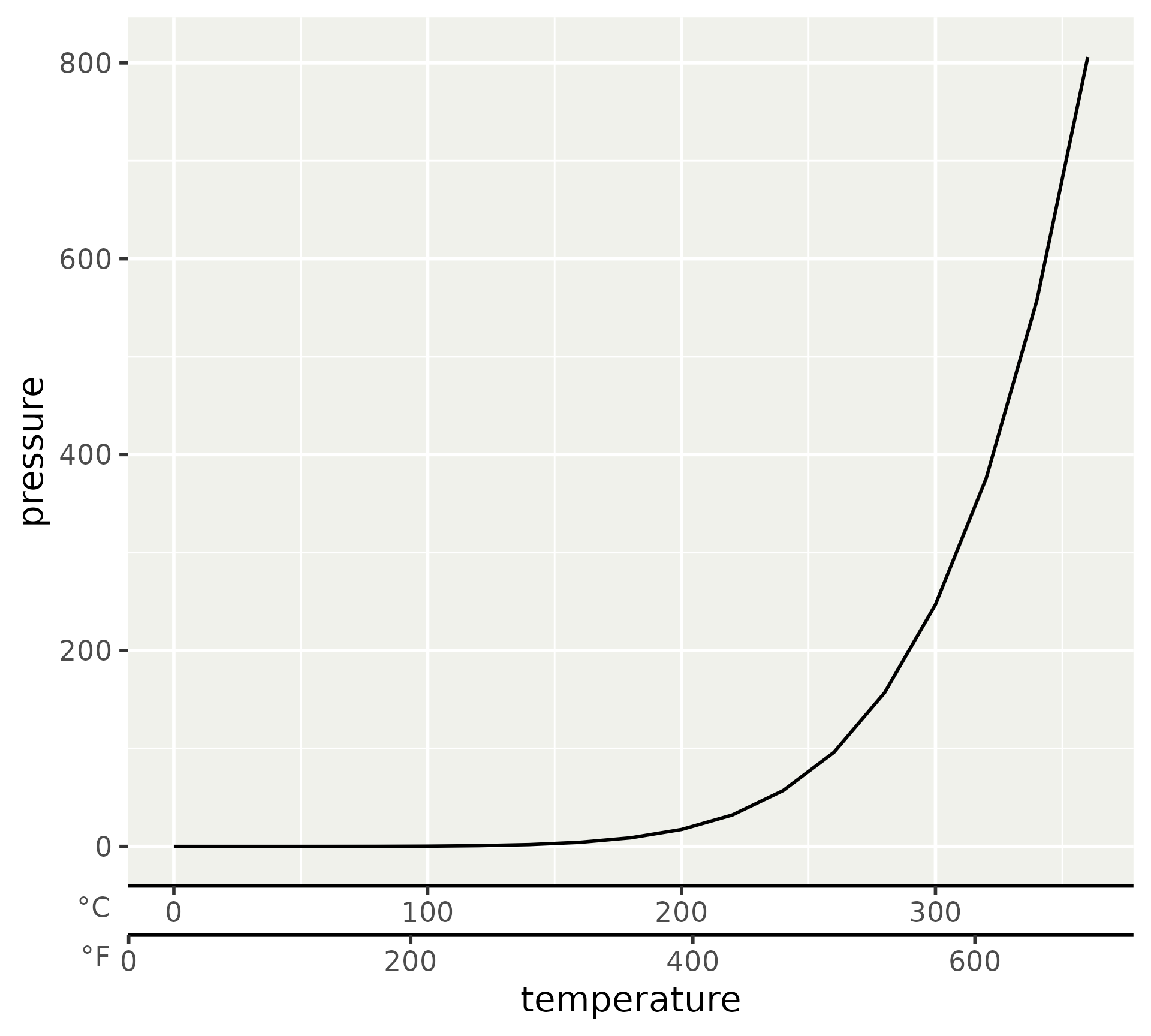
Guide extensions
In addition, many guides can be composed like stacking the Celsius and Fahrenheit guide.
stacked <- compose_stack(
  "axis",
  fahrenheit_axis,
  side.titles = c("°C", "°F")
)

p3 + guides(x = stacked)
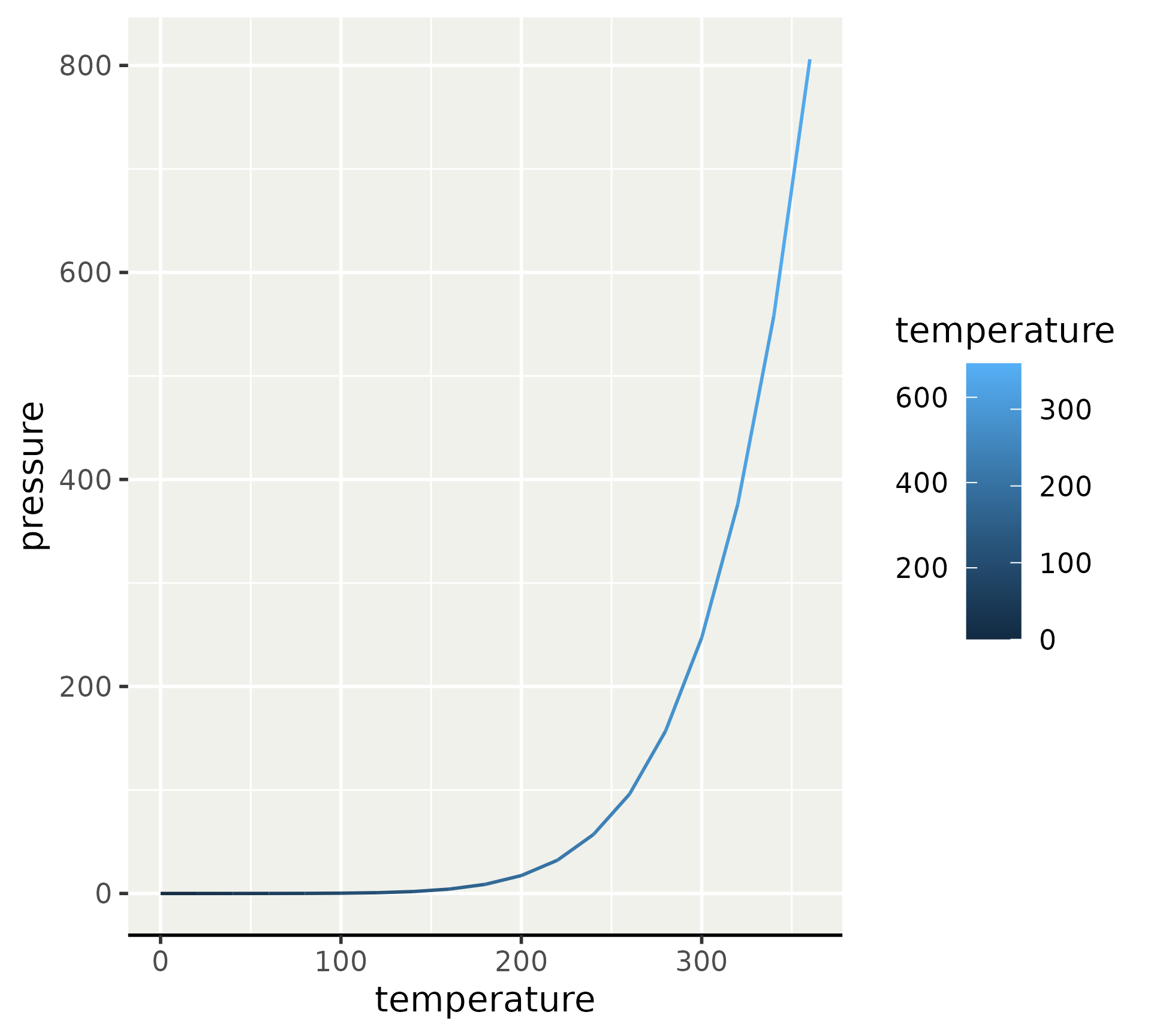
Guide extensions
legendry has re-imagined some guides as compositions.
p3 + aes(colour = temperature) +
  guides(colour = guide_colbar(
    second_guide = fahrenheit_axis,
    suppress_labels = "none"
  ))
Guide extensions
Aside from composability, re-imagined guides come with extra features.
p3 + aes(colour = temperature) +
  scale_colour_viridis_c(
    limits = c(100, 300),
    guide = "colbar"
  )
Guide extensions
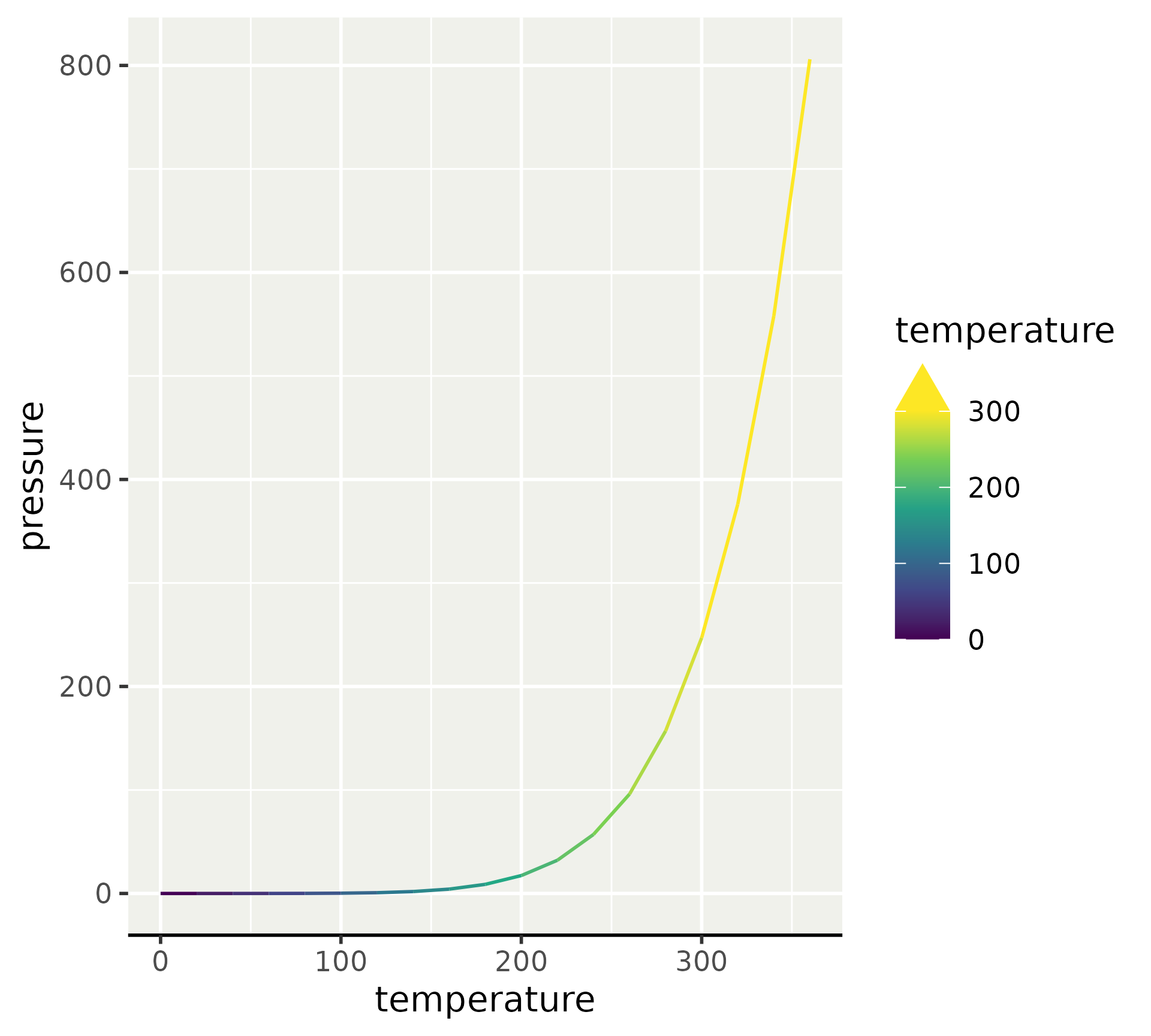
Aside from composability, re-imagined guides come with extra features.
p3 + aes(colour = temperature) +
  scale_colour_viridis_c(
    limits = c(NA, 300),
    guide = "colbar",
    oob = scales::oob_squish
  )
Custom guides: summary
- Guides give your plots meaning
- Guides can have local themes for individually tweaking them
- Guide extensions, such as those in the legendry package, expand your arsenal.