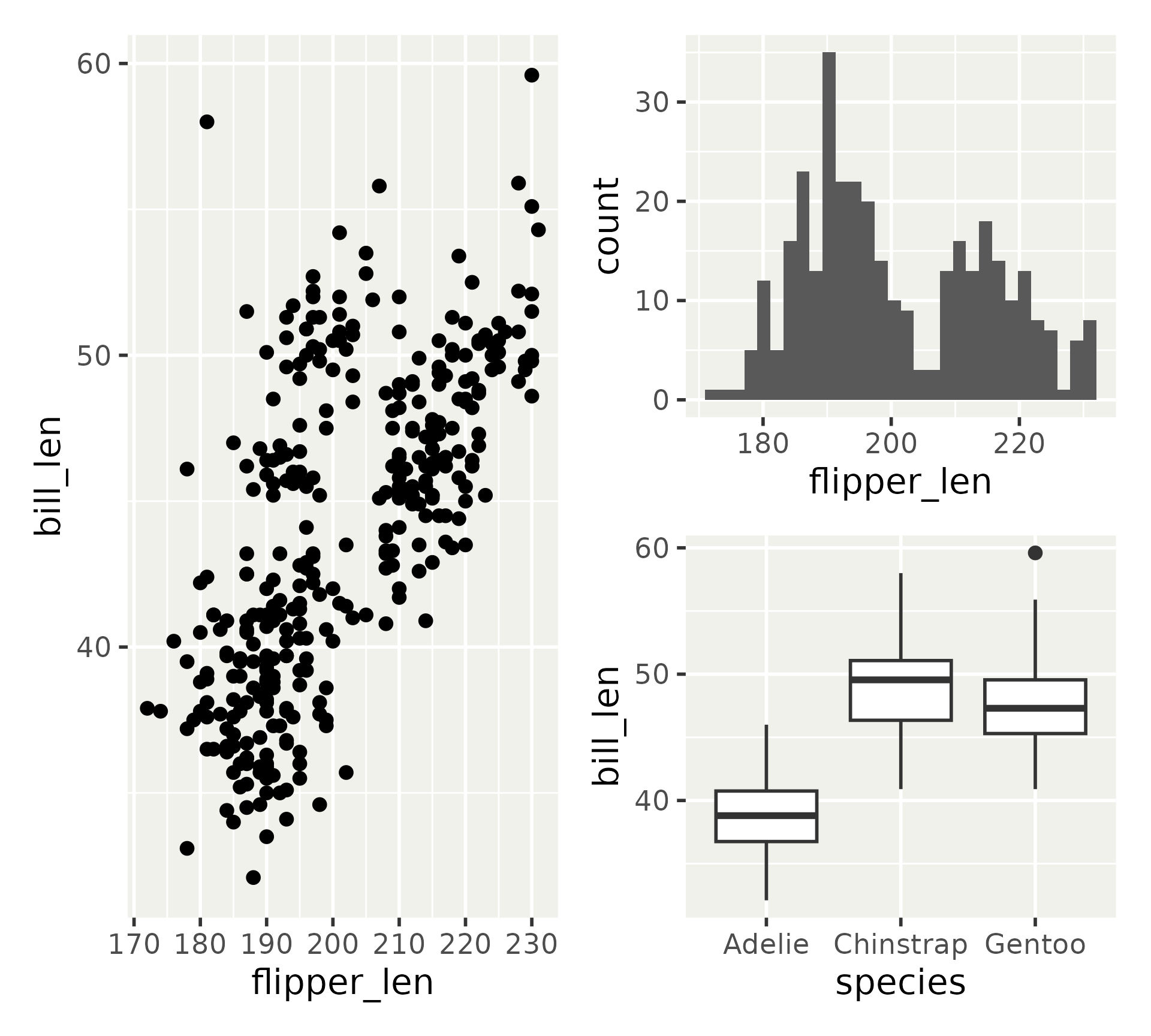
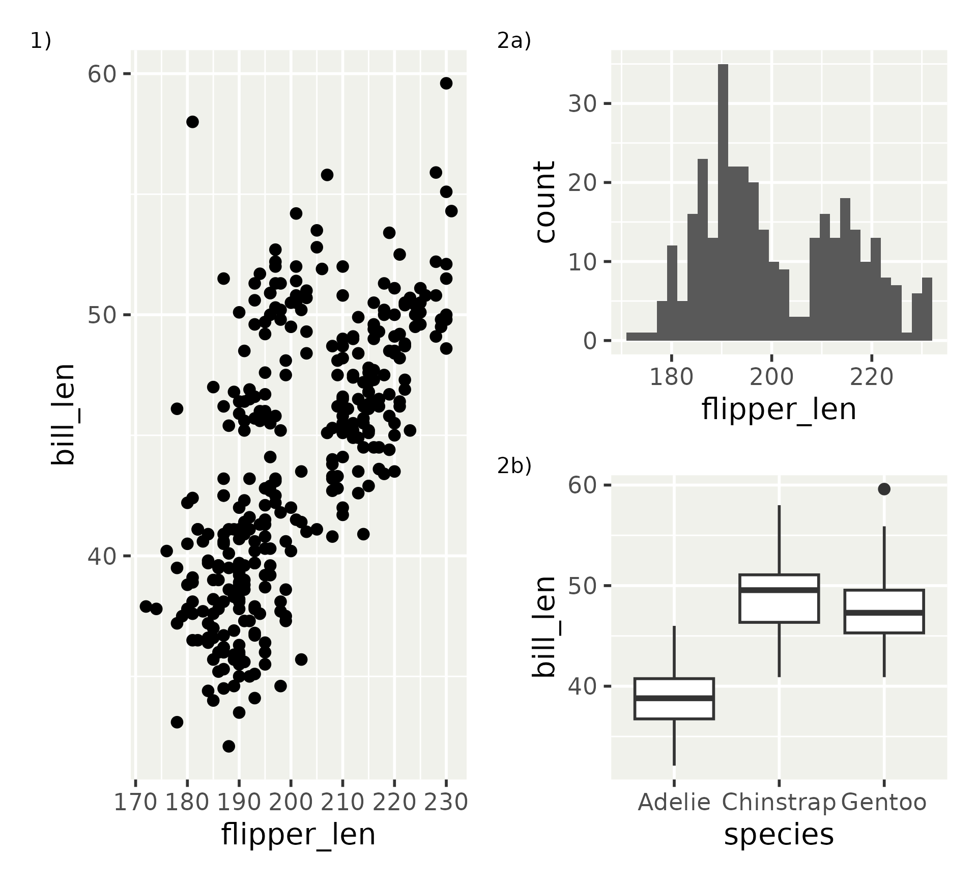
Plot composition

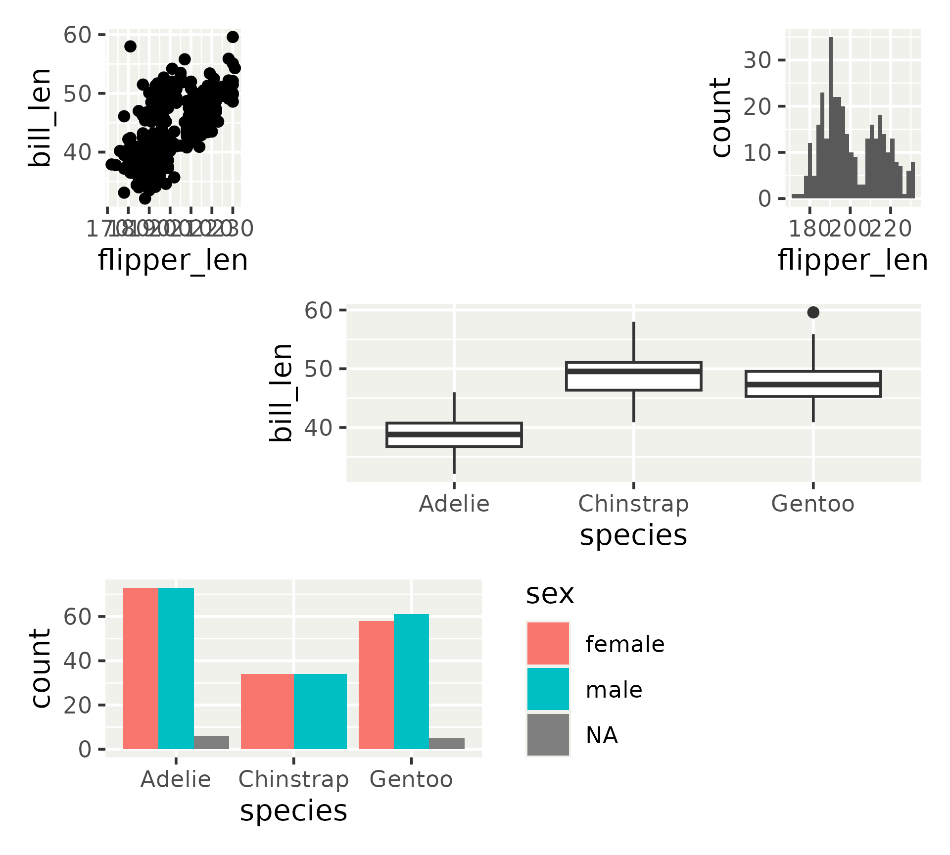
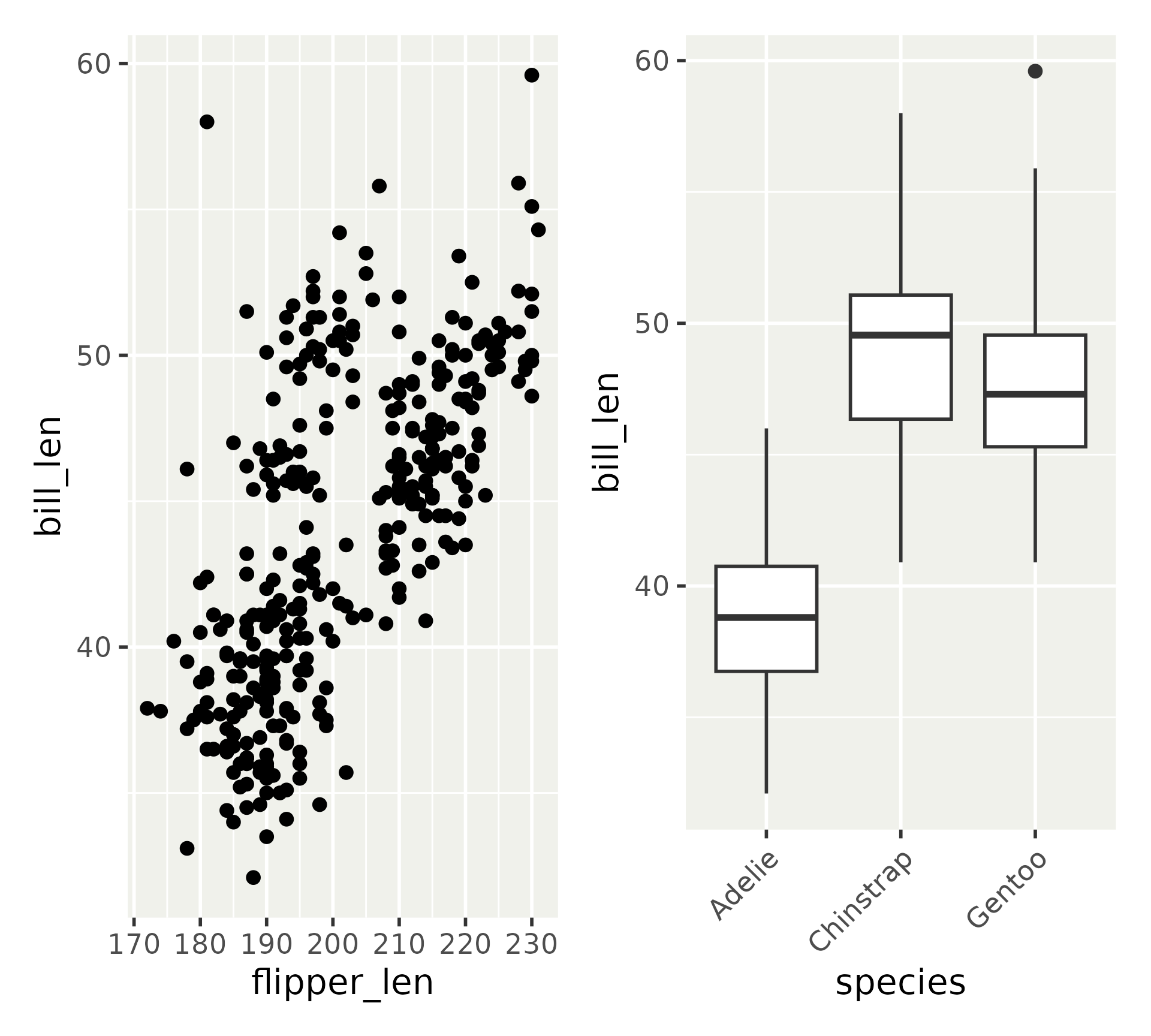
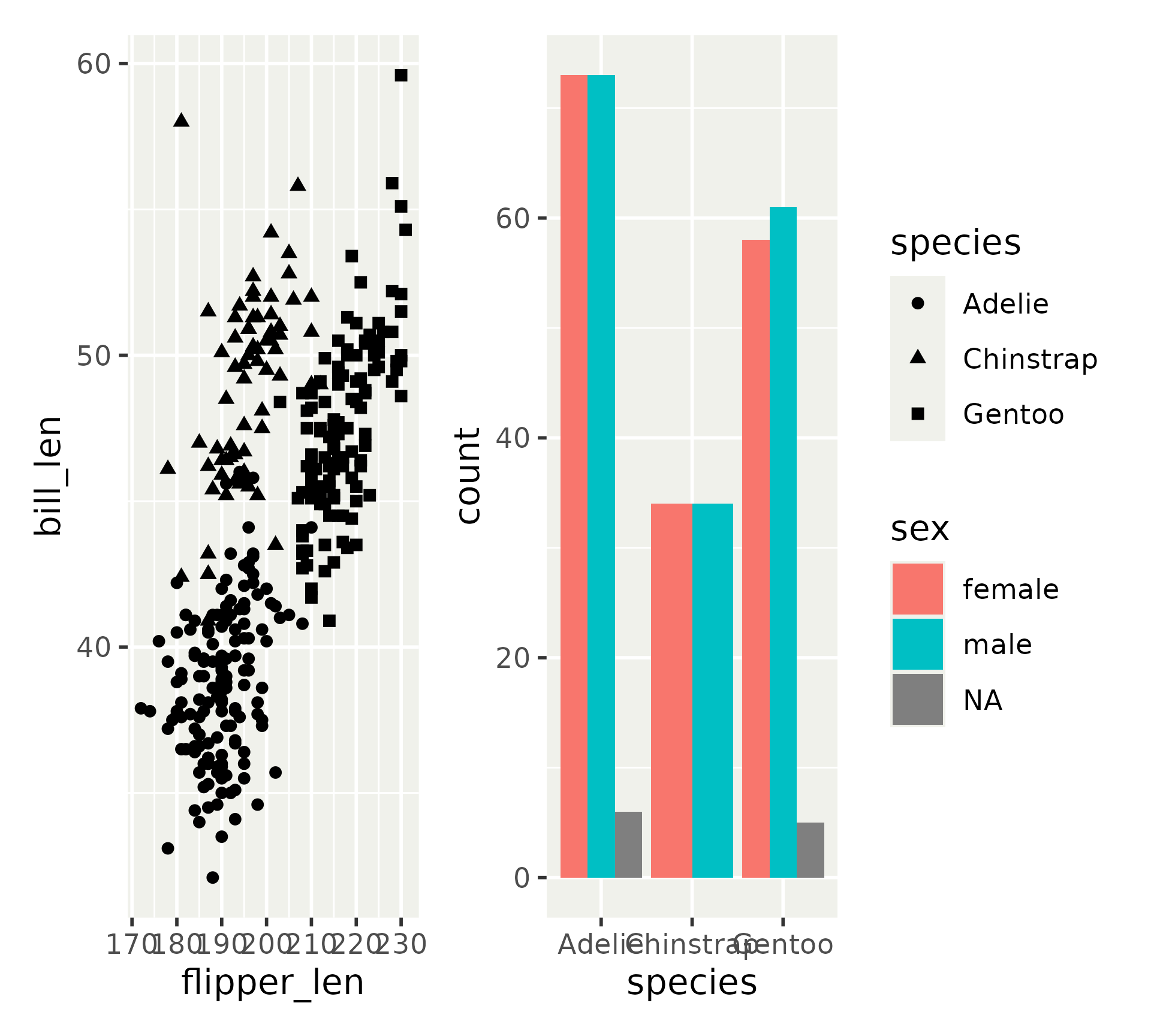
Patchwork in a nutshell

Patchwork in a nutshell
Patchwork in a nutshell
Patchwork in a nutshell

Patchwork in a nutshell
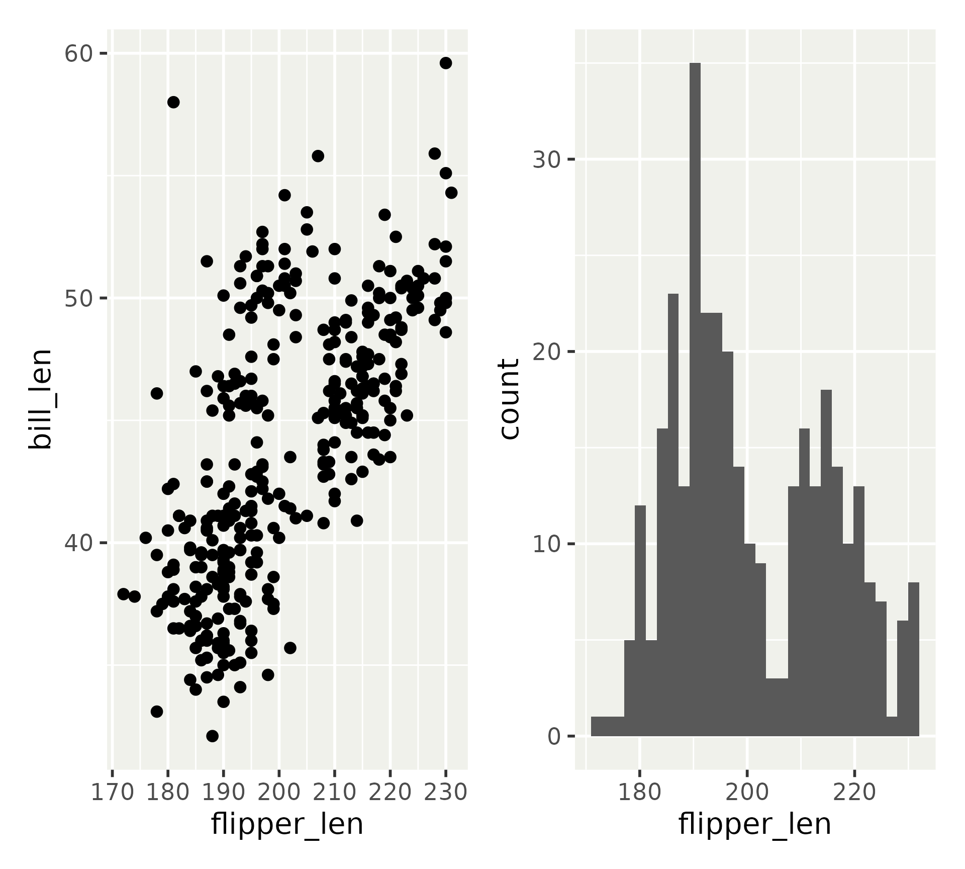
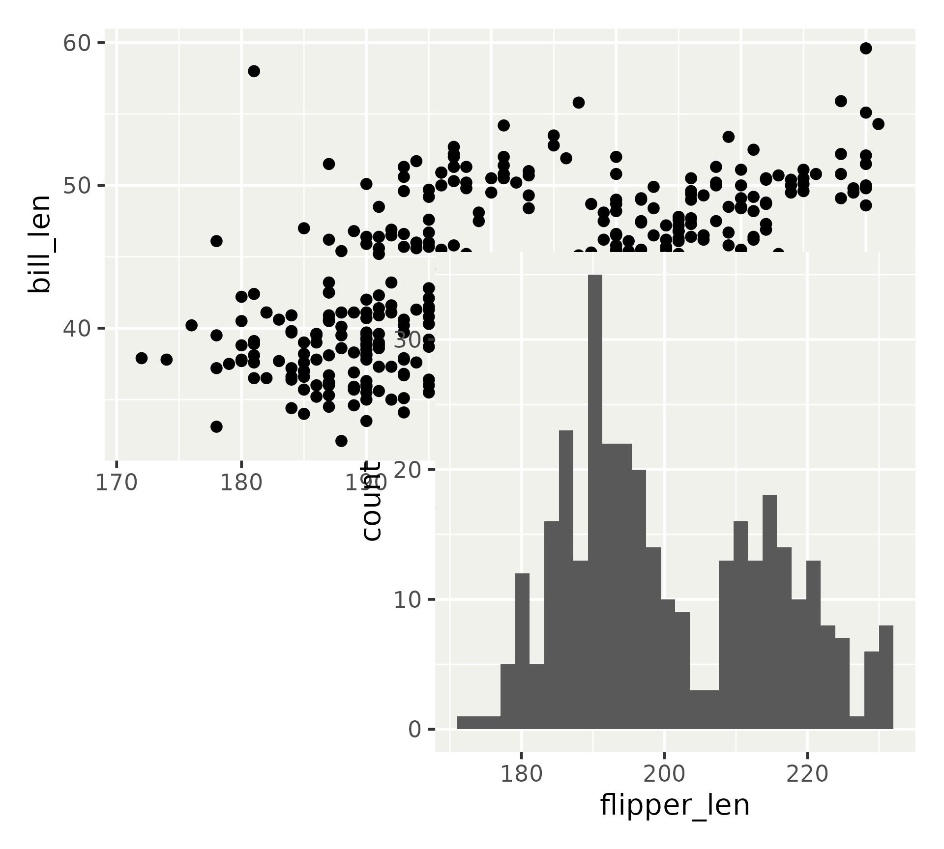
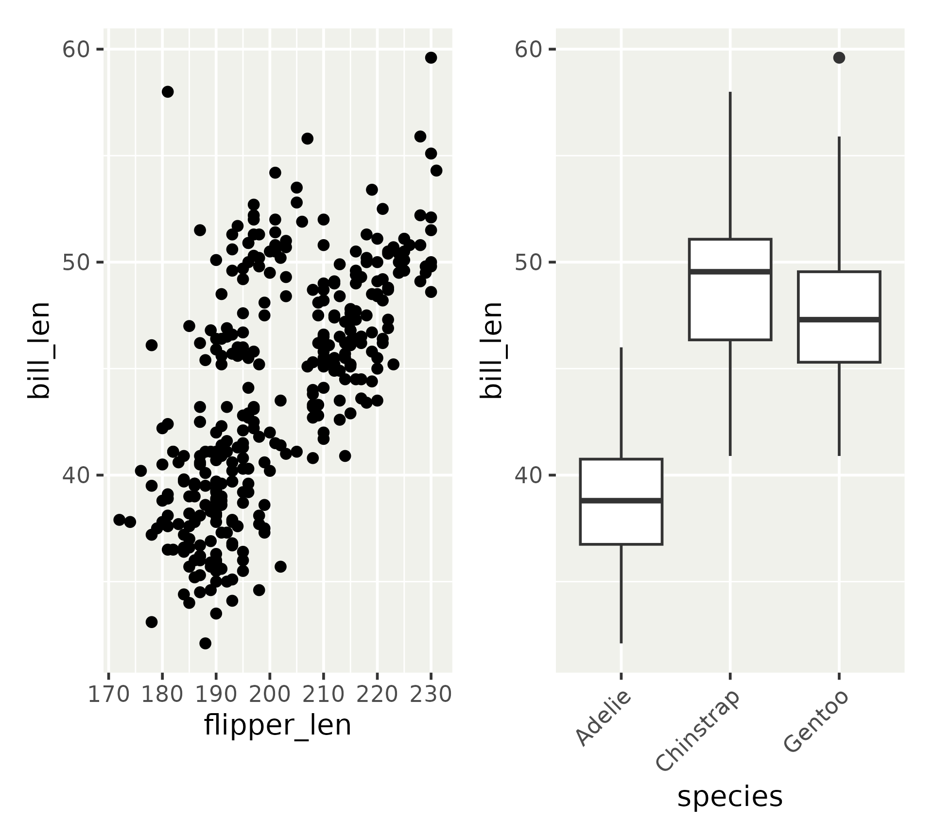
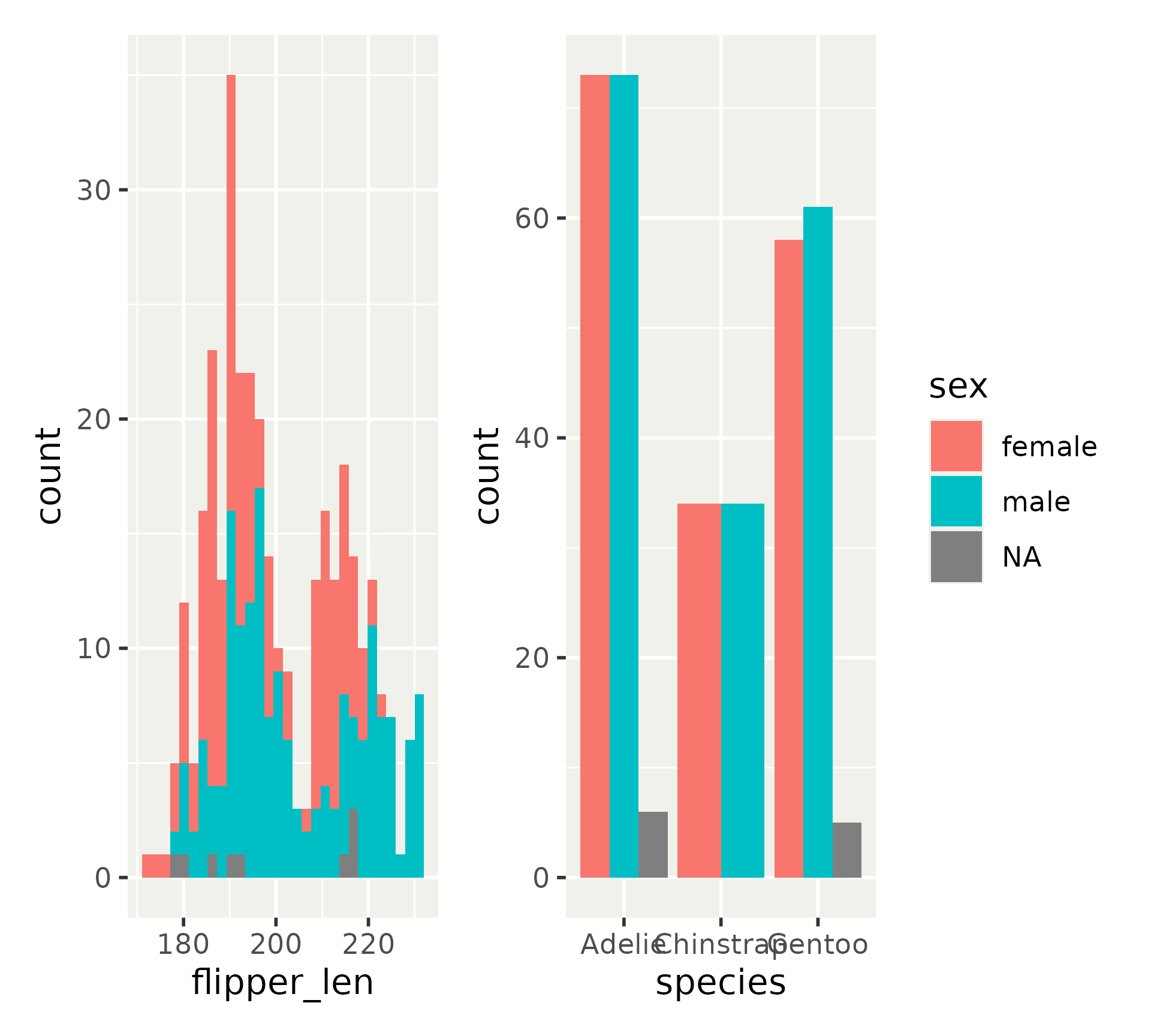
Patchwork layout model

Patchwork layout model

Patchwork layout model

Patchwork layout model

Patchwork layout model

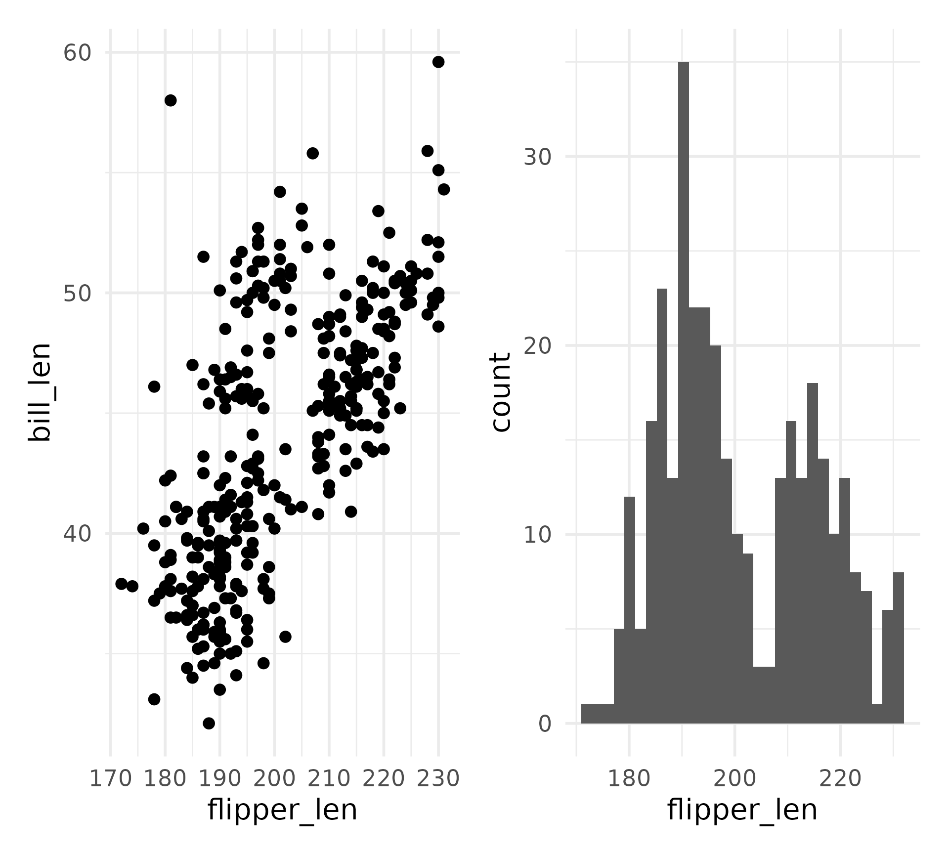
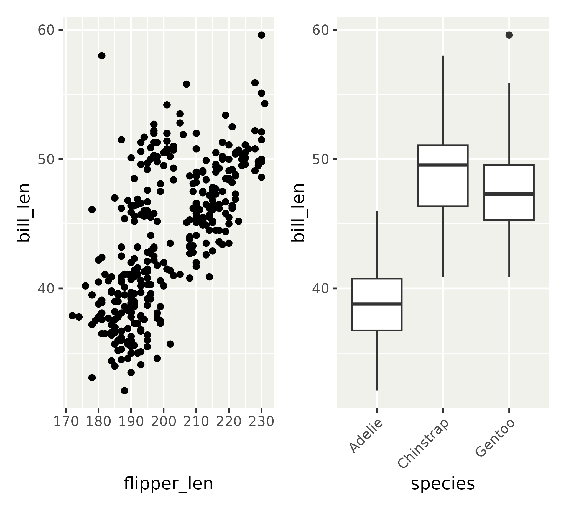
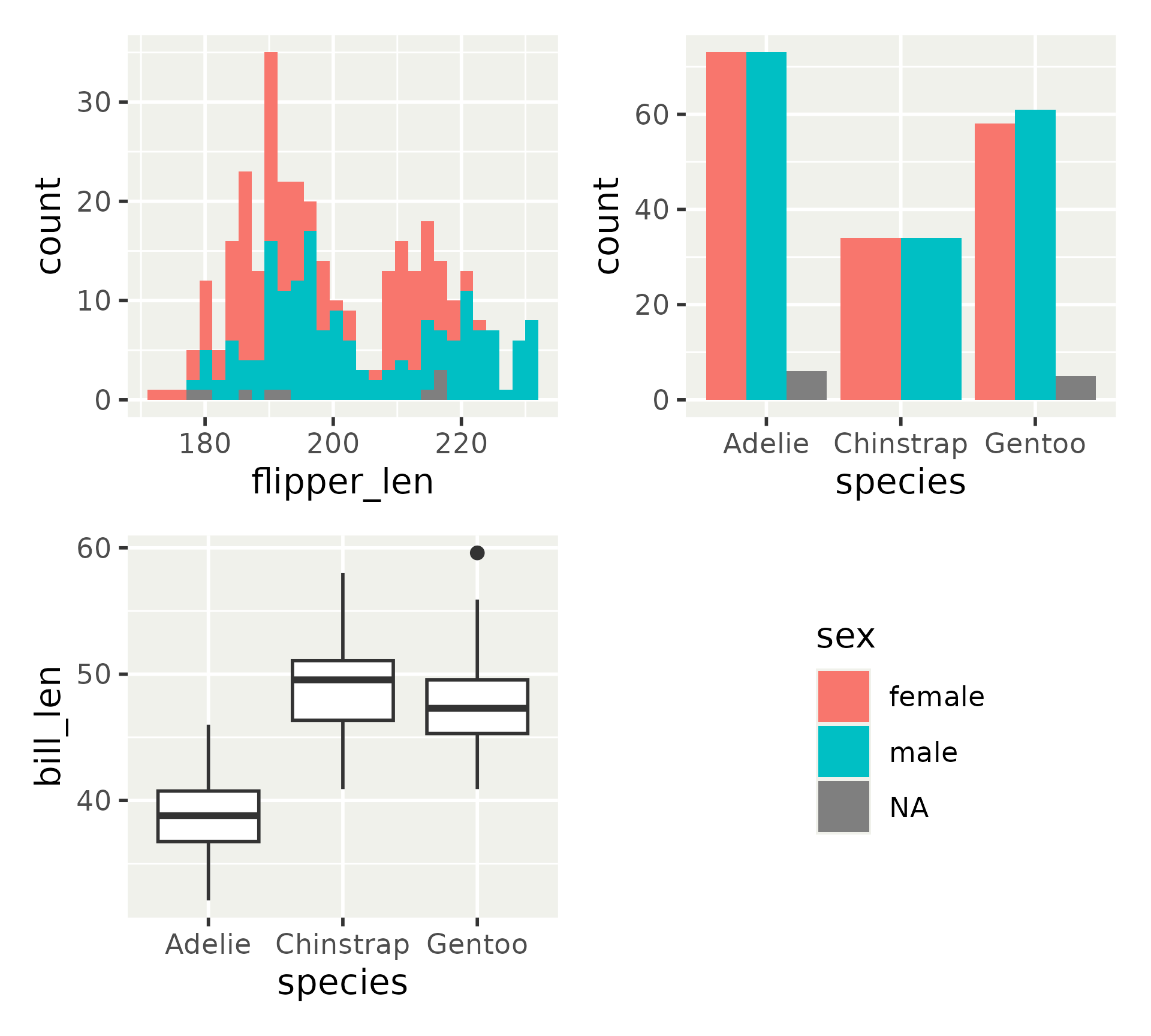
More layout options
More layout options

More layout options
More layout options
Layout modifiers - Insets
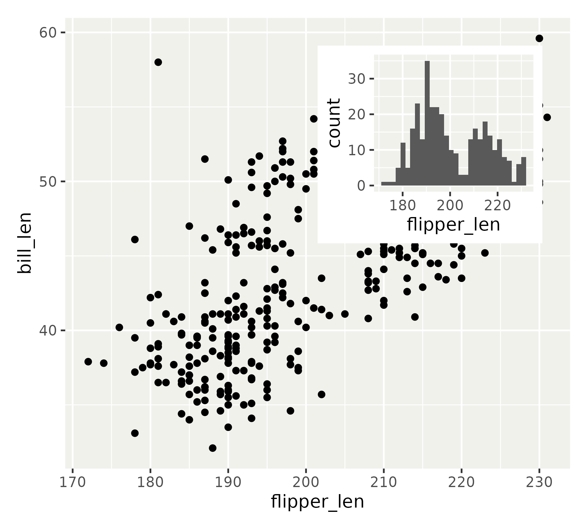
Layout modifiers - Free
Layout modifiers - Free
Layout modifiers - Free
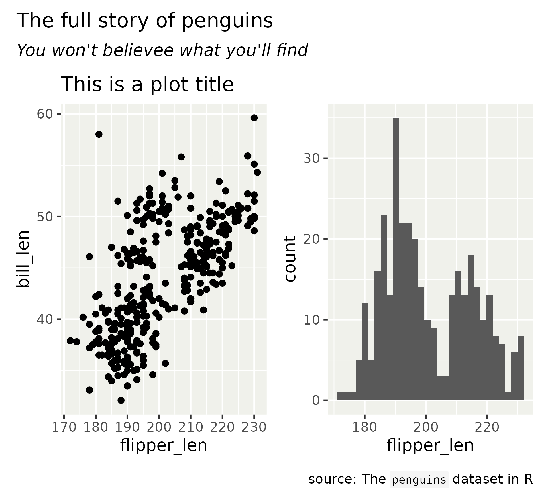
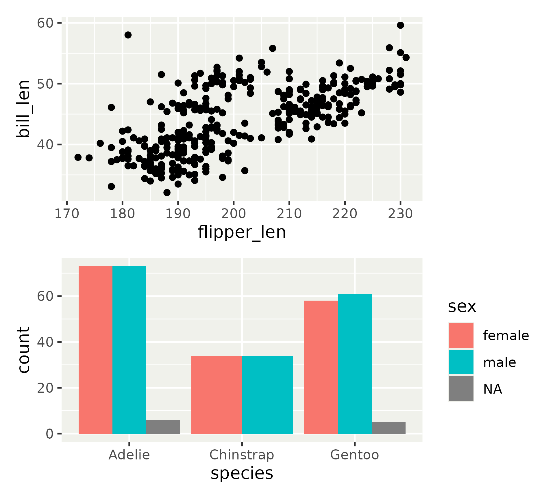
Annotations
- Once composed, the parts will constitute a new graphic
- Like the individual plots, this graphic can be annotated
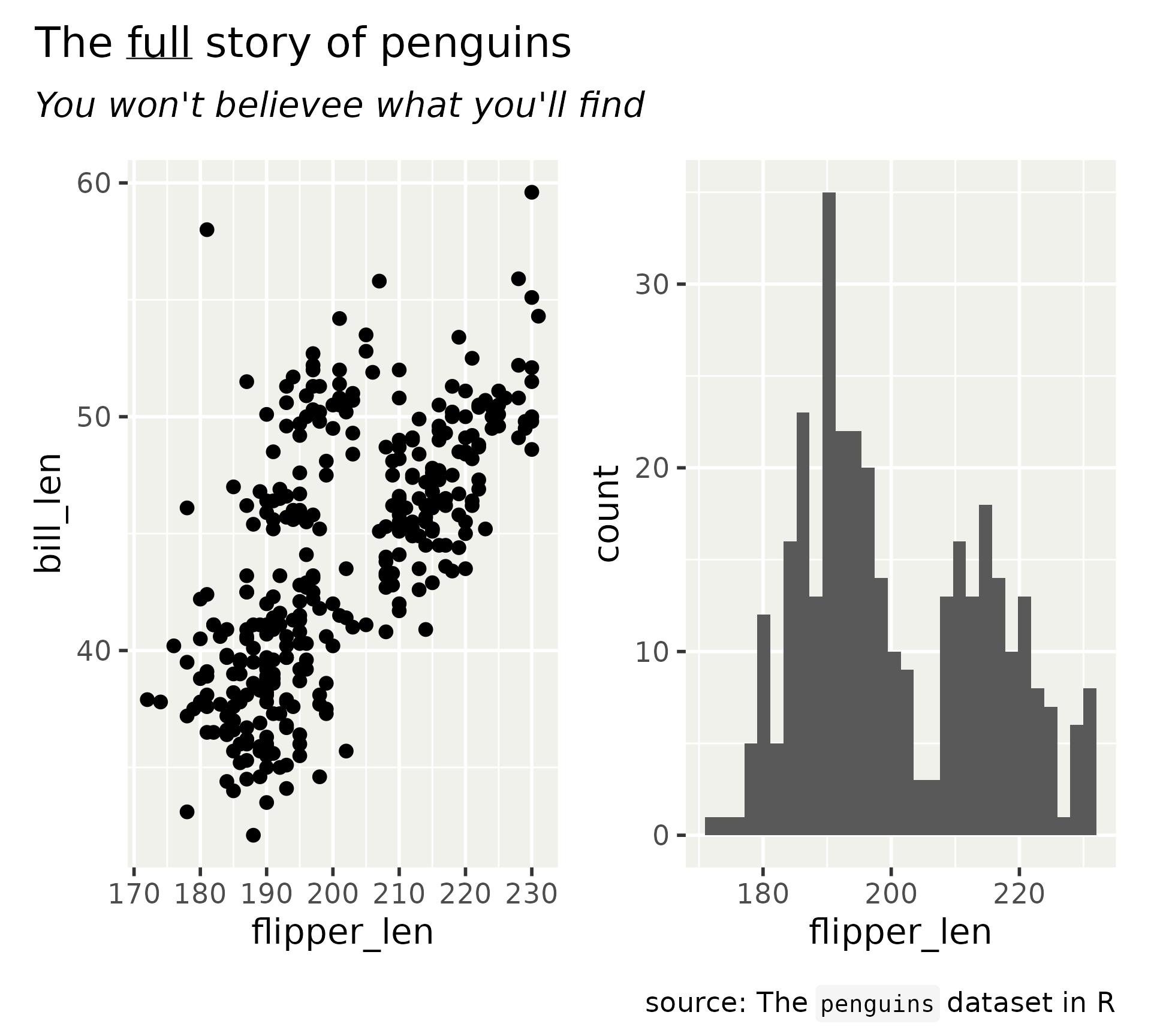
Annotations
- Once composed, the parts will constitute a new graphic
- Like the individual plots, this graphic can be annotated
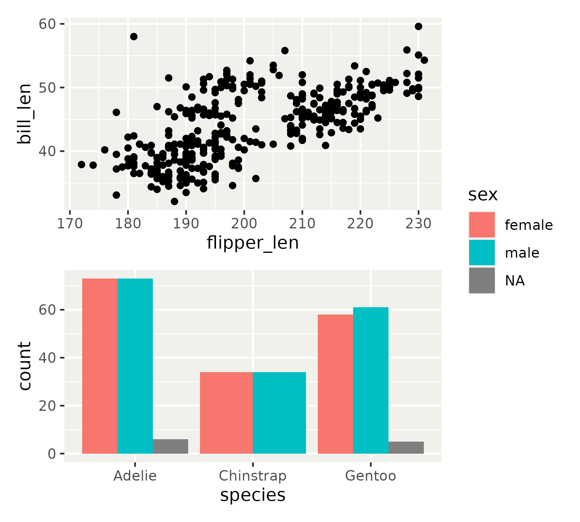
Tagging
With multi-panel graphics you often need a way to refer to the subgraphics

Tagging
It knows about nesting as well
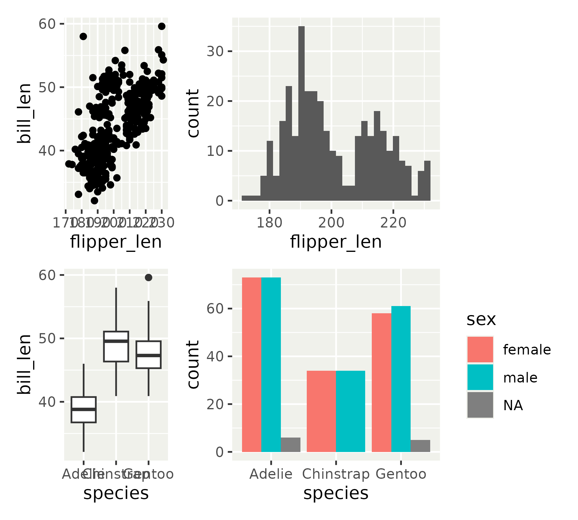
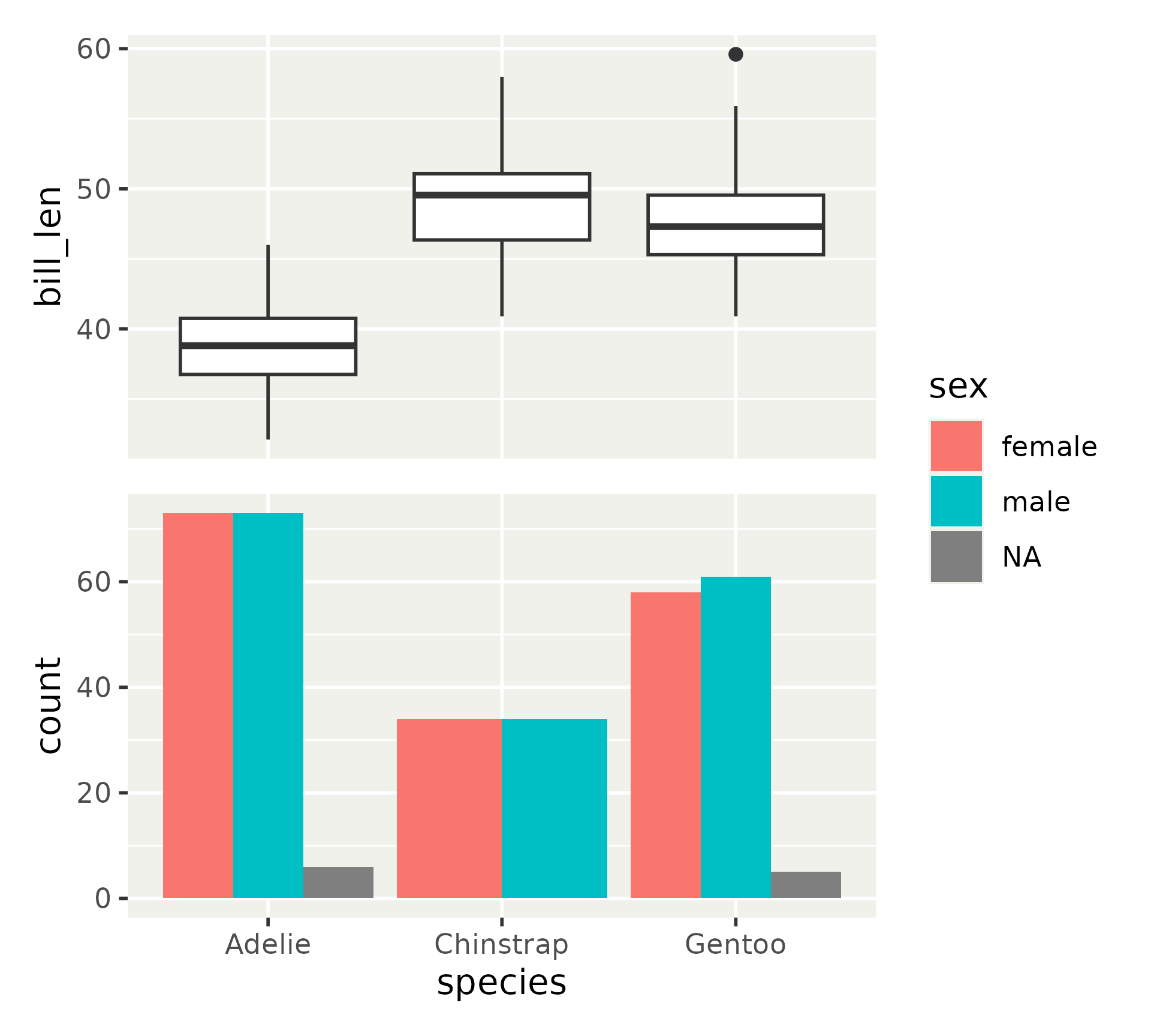
Guide handling
Guides are often global instead of linked to a single subplot
Guide handling
Use guides = "collect" to fetch all guides from subplots and place them at the top level
Guide handling
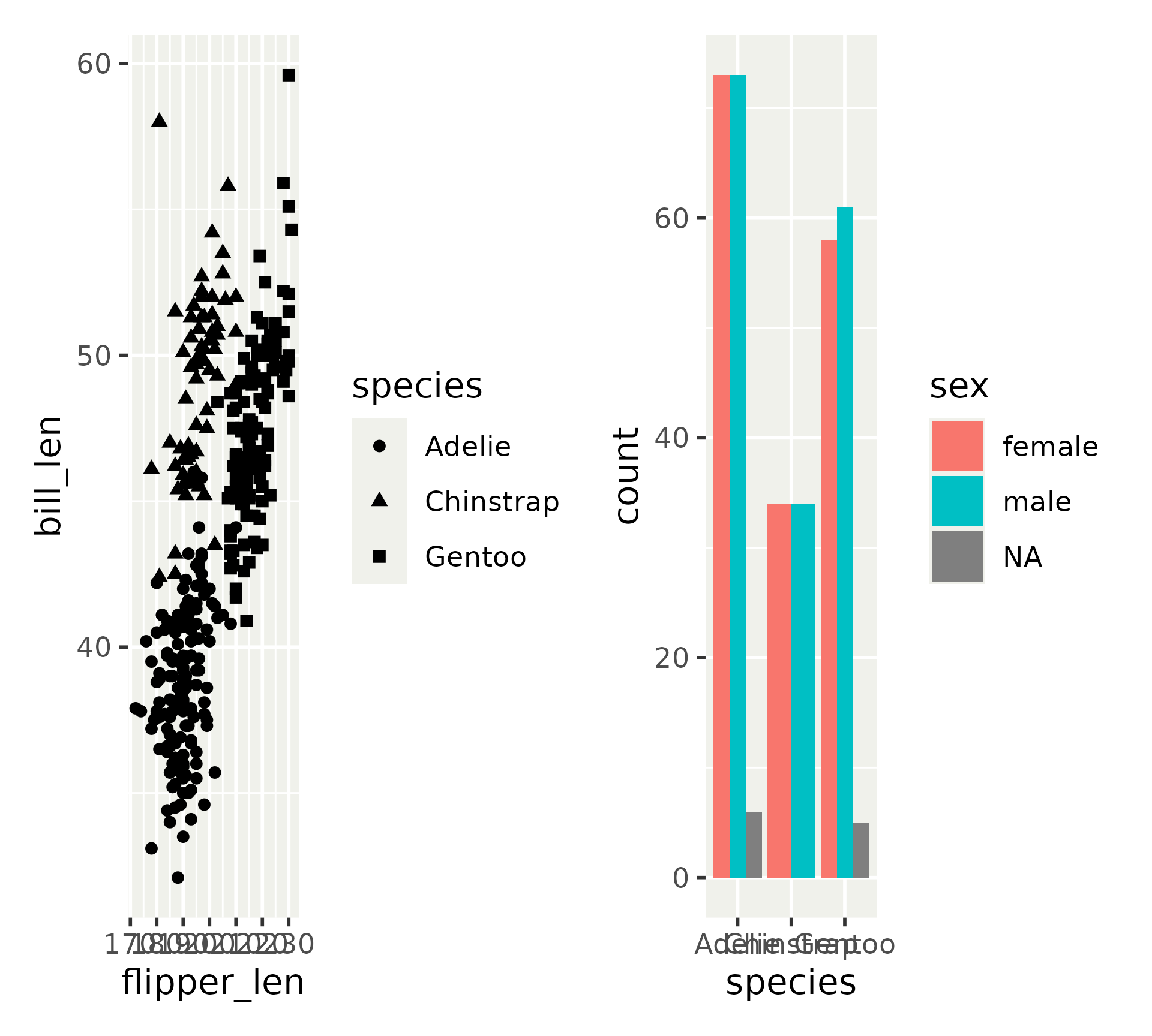
Guide handling
Guide handling
Duplicate guides are automatically removed
Guide handling
You can place guides inside the composition as well.
Guide handling
Axes are guides too
Other objects: gt
Other objects: gt
Other objects: images
Other objects: grobs
Other objects: base graphics
Other objects: base graphics
![]()