# Creating modifiable copy of StatStatGood <-ggproto(NULL, Stat)# Changing a fieldStatGood <-ggproto(NULL, Stat, required_aes ="x")Stat$required_aes## character(0)# This does NOT copy StatStatBad <- Stat# Modify-in-place shenanigansStatBad$required_aes <-"x"Stat$required_aes## [1] "x"# Never circularly define a ggproto object# Stat <- ggproto(NULL, Stat)
ggproto esoterica
Methods have access to the class object itself via a self variable if it is included as an argument in the method. It can be used to read fields and use other methods.
Stat$aesthetics## <ggproto method>## <Wrapper function>## function (...) ## aesthetics(..., self = self)## ## <Inner function (f)>## function (self) ## {## if (is.null(self$required_aes)) {## required_aes <- NULL## }## else {## required_aes <- unlist(strsplit(self$required_aes, "|", ## fixed = TRUE))## }## c(union(required_aes, names(self$default_aes)), self$optional_aes, ## "group")## }StatDensity$aesthetics()## [1] "x" "y" "fill" "weight" "group"
ggproto esoterica
Extendible classes are stateless: fields don’t mutate during plot building. State is primarily encoded in the data, and secondarily in params managed by ggplot2’s internals. Fields should be ‘read only’.
AddNumber <-ggproto("AddNumber",state =0,add =function(self, number) {# We read and write the 'state' field# Do not do this in serious code! self$state <- self$state + number self$state })AddNumber$add(10)## [1] 10AddNumber$add(5)## [1] 15
Build your own Stat
Input is evaluated aesthetics in a data frame. Output is an amended data frame with computed variables.
Define a ‘compute’ function.
Encapsulate that function in a Stat subclass.
Provide a constructor.
Defining a compute function
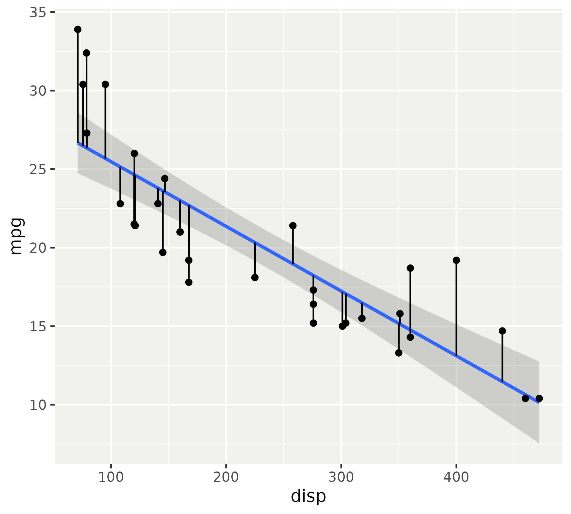
This adds fitted values and residuals from a linear model to data as computed variables. Similar to a bare bone broom::augment(). It assumes the presence of an x and y variable.
residual_lines <-function(data, formula = y ~ x, ...) { model <-lm(formula, data = data)# Create computed variables data$fitted <-predict(model) data$residual <-residuals(model) data}
Defining a compute function
You can test the compute function outside ggplot to convince yourself it is doing the right thing. Using a separate function is also easier to debug.
p <-ggplot(mtcars, aes(disp, mpg)) +geom_smooth(method ="lm", formula = y ~ x ) +geom_point()new_data <- mtcars |># Provide assumed `x` and `y` variables dplyr::mutate(x = disp, y = mpg) |>residual_lines()p +geom_segment(data = new_data,aes(yend = fitted))
Encapsulating the compute function
We create a Stat subclass using our function as the compute_group method.
StatResidual <-ggproto("StatResidual", # class name Stat, # parentcompute_group = residual_lines)p +geom_segment(stat = StatResidual)
Error in `geom_segment()`:
! Problem while setting up geom.
ℹ Error occurred in the 3rd layer.
Caused by error in `compute_geom_1()`:
! `geom_segment()` requires the following missing aesthetics: xend or
  yend.
Encapsulating the compute function
To resolve friction, we can try fixing it on the user-side.
StatResidual <-ggproto("StatResidual", # class name Stat, # parentcompute_group = residual_lines)p +geom_segment(aes(yend =after_stat(fitted)), stat = StatResidual)
Encapsulating the compute function
But in this case we can provide the missing aesthetic as a default from the computed variables.
We may need to formalise any required aesthetics, or in some cases: list optional aesthetics.
StatResidual <-ggproto("StatResidual", Stat,compute_group = residual_lines,default_aes =aes(yend =after_stat(fitted) ),# As mentioned before, the compute # function assumes the presence # of `x` and `y` variablesrequired_aes =c("x", "y"),# This example doesn't have # optional aestheticsoptional_aes =character() )p +geom_segment(stat = StatResidual)
Encapsulating the compute function
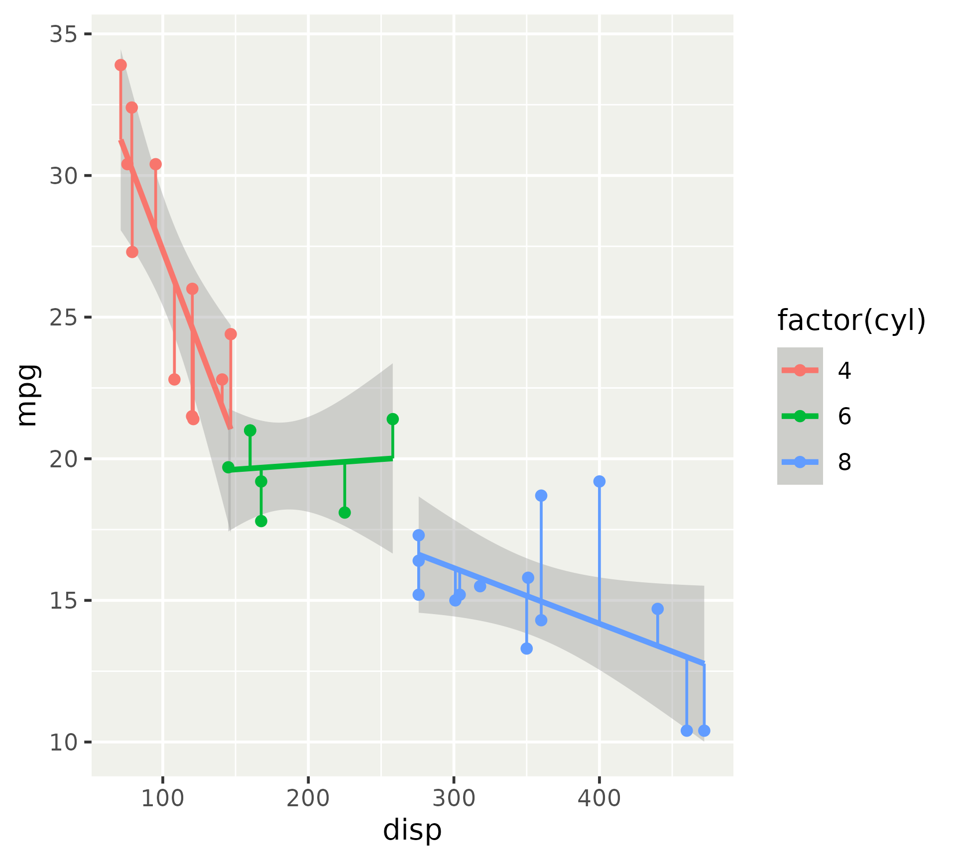
We can re-assure ourselves that our Stat behaves correctly when the data has groups.
p +geom_segment(stat = StatResidual) +aes(colour =factor(cyl))
Encapsulating the compute function
A few considerations:
use compute_group() when group-level stats are required.
use compute_panel() when computing within single panels.
by default delegates computation to compute_group()
useful when between-group computations are needed.
don’t use compute_layer() unless you have no other options.
by default delegates computation to compute_panel().
The methods can be debugged with ggplot2:::ggproto_debug(StatResidual$compute_group).
Making a constructor
A good start is to use other constructors as a template.
Typically, the first two arguments are mapping and data. Every layer needs geom, stat and position. A stat_* constructor omits the stat argument because that will be provided for you. A geom_*() constructor omits the geom argument.
2
Parameters for your Stat come after the ... argument, which requires users to write the argument names out in full.
3
The na.rm, show.legend and inherit.aes arguments come last and should have these default values in most cases. If you’re making an annotate_*() layer, you may put inherit.aes = FALSE for example.
4
You can look at the ?layer documentation to see what are the standard arguments.
5
We’re using rlang::list2() because it supports argument splicing.
6
The na.rm argument, all parameters to the Stat and ... gets passed to the layer(params) argument.
7
Note that in a stat_*() constructor, the layer(stat) argument is fixed. In a geom_*() constructor, the layer(geom) argument is fixed.
Making a constructor
When we make our own constructor, we follow the same rules.
Typically, the first two arguments are mapping and data. Every layer needs geom, stat and position. A stat_* constructor omits the stat argument because that will be provided for you. A geom_*() constructor omits the geom argument.
2
Parameters for your Stat come after the ... argument, which requires users to write the argument names out in full.
3
The na.rm, show.legend and inherit.aes arguments come last and should have these default values in most cases. If you’re making an annotate_*() layer, you may put inherit.aes = FALSE for example.
4
You can look at the ?layer documentation to see what are the standard arguments.
5
We’re using rlang::list2() because it supports argument splicing.
6
The na.rm argument, all parameters to the Stat and ... gets passed to the layer(params) argument.
7
Note that in a stat_*() constructor, the layer(stat) argument is fixed. In a geom_*() constructor, the layer(geom) argument is fixed.
Making a constructor
Instead of following all the rules, you can also use cookie-cutter make_constructor().
stat_residual <-make_constructor(StatResidual, geom ="segment")print(stat_residual)## function (mapping = NULL, data = NULL, geom = "segment", position = "identity", ## ..., formula = y ~ x, na.rm = FALSE, show.legend = NA, inherit.aes = TRUE) ## {## layer(mapping = mapping, data = data, geom = geom, stat = "residual", ## position = position, show.legend = show.legend, inherit.aes = inherit.aes, ## params = list2(na.rm = na.rm, formula = formula, ...))## }## <environment: 0x560775a0df18>p +stat_residual()
Additional considerations
You can use the setup_params() for:
Sanity checking
stat_smooth() tries to find valid method.
stat_bin() watches for deprecated arguments.
Initiating layer-level parameters
stat_contour() tracks range of z aesthetic to re-use in group-level computation.
Setting up orientation
Most bidirectional stats
StatContour$setup_params## <ggproto method>## <Wrapper function>## function (...) ## setup_params(...)## ## <Inner function (f)>## function (data, params) ## {## params$z.range <- range(data$z, na.rm = TRUE, finite = TRUE)## params## }
Additional considerations
You can use the setup_data() method for:
Data wrangling at the layer-level
stat_boxplot() removes NA values.
Initiating optional aesthetics
Sanity checking
stat_contour() cannot have duplicate data.
StatBoxplot$setup_data## <ggproto method>## <Wrapper function>## function (...) ## setup_data(..., self = self)## ## <Inner function (f)>## function (self, data, params) ## {## data <- flip_data(data, params$flipped_aes)## data$x <- data$x %||% 0## data <- remove_missing(data, na.rm = params$na.rm, vars = "x", ## name = "stat_boxplot")## flip_data(data, params$flipped_aes)## }